Jim Sanborn couldn’t consider it. He was weeks away from auctioning off the reply to Kryptos, the sculpture he created for the CIA that had defied resolution for 35 years. As all the time, wannabe solvers saved on paying him a $50 payment to supply their guesses to the remaining unsolved portion of the 1,800-character encrypted message, often known as K4—incorrect with out exception. Then, on September 3, he opened an e-mail from the newest applicant, Jarett Kobek, which began, “I consider the textual content of K4 is as follows …” He’d seen phrases like this 1000’s of occasions earlier than. However this time, the textual content was right.
“I used to be in shock,” Sanborn tells me. “Actual severe shock.” The timing was terrible. Sanborn, who turns 80 this yr, noticed the public sale as a method for somebody to proceed his work of vetting potential options whereas sustaining the thriller of Kryptos. He’d additionally been trying ahead to getting compensated for his work. What got here subsequent was much more shattering. He rapidly bought on the cellphone with Kobek and his good friend Richard Byrne, who gobsmacked him by reporting they didn’t discover the answer by codebreaking. As an alternative, Kobek had realized from the public sale discover that some Kryptos supplies had been held on the Smithsonian’s Archives of American Artwork in Washington, DC. Kobek, a California novelist (considered one of his books known as I Hate the Web), bought his good friend, the playwright and journalist Byrne, to {photograph} among the holdings. To Kobek’s astonishment, two of the photographs contained a 97-character passage with phrases that Sanborn had beforehand dropped as clues. He was staring on the full unencrypted textual content that CIA and NSA codebreakers, together with numerous teachers and hobbyists, had sought for many years.
The key of Kryptos was out of the artist’s fingers, in essentially the most humiliating method possible—Sanborn himself had mistakenly submitted it in readable kind to the museum. For 35 years the Kryptos plaintext had been a summit that none had reached. Abruptly some had attained it—not by climbing to the height however by hitching a trip to the highest. Sanborn’s grand imaginative and prescient for a bit of artwork that illuminated the thought of secrecy itself was imperiled—as was the public sale. Now he had to determine what to do about it.
Enter: The Media
The preliminary cellphone name had been pleasant. Kobek and Byrne insisted that they didn’t wish to mess up the public sale. After he hung up, Sanborn known as the public sale home. That’s when issues began going sideways. As Sanborn tells me, “They mentioned, ‘Hear, see if the blokes will signal NDAs, and see if they’re going to take a portion of the proceeds.’ And I mentioned, ‘Oh geez, man, I do not find out about that. However I supplied it.’”
Kobek and Byrne had been uncomfortable with that association and refused to signal. (RR Public sale govt vice chairman Bobby Livingston didn’t touch upon the authorized subject however says of an NDA, “It’s one thing that will be comforting to our shoppers.”) Sanborn advised them his intent was to get the Smithsonian to freeze the archives—which it did. He assumed Kobek and Byrne would keep silent. “In the event you do not launch it, you are heroes to me,” Sanborn advised them.
“I believed all the pieces was OK,” he says, “After which hastily [the journalist] John Schwartz calls me and says these guys wish to publish it in The New York Instances.” Kobek explains to me that they contacted Schwartz partially to alleviate some authorized stress. “There was risk after risk being despatched to us from the public sale home’s attorneys, threatening to sue us for a mess of issues,” he says. (After I ask Livingston if his attorneys have been contacting Kobek, he says, “There’s attorneys speaking to one another,” and provides that there could be copyright considerations if Kobek and Byrne printed the plaintext.) On October 16, Schwartz printed his scoop, informing the world that the plaintext was out.
Sanborn tells me that Kobek shared the plaintext with Schwartz over the cellphone. When requested about this, Kobek says, “I can’t discuss that…I’m underneath important authorized peril.” Schwartz says. “As soon as my editors determined it could not be revealed within the story, I deleted the textual content from my interviews file. I don’t understand it.” (So don’t bug him.)
Center class earnings is a variety that relies on how a lot folks make the place you reside. So if earnings leans increased in a single state than in one other, the middle-income vary displays that. It additionally relies on how many individuals are within the family.
Right here is how middle-income varies throughout the states and the nation total.
Family Center Revenue
Bars characterize a variety for every state, sorted by median and adjusted for family dimension.
That is based mostly on knowledge from the five-year American Group Survey from 2023. The newer 2024 knowledge was presupposed to be out by now, so I’ll replace when the federal authorities will get their act collectively.
I’m utilizing the Pew Analysis definition of center earnings, which is two-thirds the median to twice the median.
Washington, D.C. is on the prime, as you would possibly count on for a metropolis, however the median earnings for a family with 5 folks was decrease than for a family of 4. Anomaly? Demographic distinction between four- and five-person households? I’m unsure about this.
However holy cannoli, Massachusetts. A $300,000 earnings places you in center class for a family of 4. Right here I assumed California was inflated, however I assume it’s a much bigger state, which provides extra space for variation in smaller cities and rural areas. Massachusetts appears extra concentrated in Boston. It’s most likely the same story with New Jersey, Maryland, Connecticut, and New Hampshire.
1. Can I get schistosomiasis from swimming swimming pools?
No, schistosomiasis just isn’t transmitted in chlorinated swimming swimming pools. The parasite wants particular freshwater snails to finish its life cycle.
2. Why is schistosomiasis (bilharzia) additionally referred to as swimmer’s itch?
Schistosomiasis known as “swimmer’s itch” as a result of it causes an itchy rash when parasite larvae from contaminated freshwater penetrate the pores and skin. These larvae, launched by snails, set off an allergic response, resulting in the attribute itch. Whereas not all instances result in full-blown schistosomiasis, the early rash provides it the identify.
3. Why is schistosomiasis referred to as bilharzia?
Schistosomiasis known as bilharzia after Theodor Bilharz, the German doctor who first found the parasitic worms inflicting the illness in 1851. He recognized the worms in sufferers in Egypt whereas finding out tropical ailments. The identify honors his contribution to understanding the parasite’s life cycle and its influence on human well being.
4. Is there a vaccine for schistosomiasis?
At present, there isn’t any vaccine out there for schistosomiasis. Prevention focuses on avoiding publicity and treating contaminated people.
5. Can schistosomiasis be fully cured?
Sure, when recognized and handled early, schistosomiasis might be successfully cured with praziquantel. Nonetheless, reinfection is feasible if uncovered once more.
6. How lengthy can somebody have schistosomiasis with out realizing it?
Folks can harbor the parasite for years with out extreme signs, which is why it’s typically referred to as a “silent” illness.
7. Does schistosomiasis unfold from individual to individual?
No, schistosomiasis can’t be straight transmitted from one individual to a different. The parasite must undergo its life cycle in water and snails earlier than it could infect people once more.
Trendy CSS has nice methods to place and transfer a bunch of parts relative to one another, equivalent to anchor positioning. That stated, there are cases the place it could be higher to take up the outdated methods for a little bit animation, saving effort and time.
We’ve at all times been capable of have an effect on a component’s construction, like resizing and rotating it. And after we change a component’s intrinsic sizing, its kids are affected, too. That is one thing we will use to our benefit.
Let’s say a number of circles want to maneuver in direction of and throughout each other. One thing like this:
Our markup is likely to be so simple as a factor that incorporates 4 youngster .circle parts:
So far as rotating issues, there are two choices. We will (1) animate the mum or dad container, or (2) animate every .circle individually.
Tackling that first choice might be finest as a result of animating every .circle requires defining and setting a number of animations moderately than a single animation. Earlier than we try this, we must make it possible for every .circle is contained within the factor after which completely place every one within it:
It appears to be like like we’re animating 4 circles, however what we’re actually doing is rotating the mum or dad container and altering its width, which rotates and squishes all of the circles in it as effectively:
Every .circle is mounted to a respective nook of the mum or dad with absolute positioning. When the animation is triggered within the mum or dad factor — i.e. will get the .animate class when the button is clicked — the width shrinks and it rotates 90deg. That shrinking pulls every .circle nearer to the factor’s heart, and the rotation causes the circles to change locations whereas passing by way of each other.
This method makes for a better animation to craft and handle for easy results. You’ll be able to even layer on the animations for every particular person factor for extra variations, equivalent to two squares that cross one another in the course of the animation.
/* Utilized on  (the mum or dad factor) */
.animate {
  rework:  skewY(30deg) rotateY(180deg);
  transition: 1s rework .2s;

  .sq. {
    rework: skewY(30deg);
    transition: inherit;
  }
}
See that? The mum or dad factor makes a 30deg skew and flip alongside the Y-axis, whereas the 2 youngster .sq. parts counter that distortion with the identical skew. The result’s that you simply see the kid squares flip positions whereas shifting away from one another.
If we would like the squares to kind a separation with out the flip, right here’s a method to try this:
/* Utilized on  (the mum or dad factor) */
.animate {
  rework:  skewY(30deg);
  transition: 1s rework .2s;

  .sq. {
    rework: skewY(-30deg);
    transition: inherit;
  }
}
This time, the factor is skewed 30deg, whereas the .sq. kids cancel that with a -30deg skew.
Setting skew() on a mum or dad factor helps rearrange the youngsters past what typical rectangular geometry permits. Any change within the mum or dad could be complemented, countered, or cancelled by the youngsters relying on what impact you’re on the lookout for.
Right here’s an instance the place scaling is concerned. Discover how the factor’s skewY() is negated by its kids and scale()s at a distinct worth to offset it a bit.
/* Utilized on  (the mum or dad factor) */
.animate {
  rework: rotate(-180deg) scale(.5) skewY(45deg) ;
  transition: .6s .2s;
  transition-property: rework, border-radius;

  .squares {
    rework: skewY(-45deg) scaleX(1.5);
    border-radius: 10px;
    transition: inherit;
  }
}
The mum or dad factor () rotates counter-clockwise (rotate(-180deg)), scales down (scale(.5)), and skews vertically (skewY(45deg)). The 2 kids (.sq.) cancel the mum or dad’s distortion by utilizing the unfavorable worth of the mum or dad’s skew angle (skewY(-45deg)), and scale up horizontally (scaleX(1.5)) to vary from a sq. to a horizontal bar form.
There are loads of these combos you may provide you with. I’ve made a number of extra under the place, as an alternative of triggering the animation with a JavaScript interplay, I’ve used a
factor that triggers the animation when it’s in an [open] state as soon as the factor is clicked. And every incorporates an .icon youngster demonstrating a distinct animation when the toggles between open and closed.
Click on on a
to toggle it open and closed to see the animations in motion.
That’s all I needed to share — it’s straightforward to overlook that we get some affordances for writing environment friendly animations if we contemplate how remodeling a mum or dad factor intrinsically impacts the dimensions, place, and orientation. That method, for instance, there’s no want to put in writing complicated animations for every particular person youngster factor, however moderately leverage what the mum or dad can do, then modify the habits on the youngster stage, as wanted.
Manufacturing higher batteries, quicker electronics, and simpler prescribed drugs is determined by the invention of latest supplies and the verification of their high quality. Synthetic intelligence helps with the previous, with instruments that comb by means of catalogs of supplies to rapidly tag promising candidates.
However as soon as a fabric is made, verifying its high quality nonetheless entails scanning it with specialised devices to validate its efficiency — an costly and time-consuming step that may maintain up the event and distribution of latest applied sciences.
Now, a brand new AI device developed by MIT engineers may assist clear the quality-control bottleneck, providing a quicker and cheaper possibility for sure materials-driven industries.
In a research showing right now within the journal Matter, the researchers current “SpectroGen,” a generative AI device that turbocharges scanning capabilities by serving as a digital spectrometer. The device takes in “spectra,” or measurements of a fabric in a single scanning modality, reminiscent of infrared, and generates what that materials’s spectra would appear to be if it have been scanned in a wholly totally different modality, reminiscent of X-ray. The AI-generated spectral outcomes match, with 99 % accuracy, the outcomes obtained from bodily scanning the fabric with the brand new instrument.
Sure spectroscopic modalities reveal particular properties in a fabric: Infrared reveals a fabric’s molecular teams, whereas X-ray diffraction visualizes the fabric’s crystal constructions, and Raman scattering illuminates a fabric’s molecular vibrations. Every of those properties is important in gauging a fabric’s high quality and usually requires tedious workflows on a number of costly and distinct devices to measure.
With SpectroGen, the researchers envision {that a} variety of measurements may be made utilizing a single and cheaper bodily scope. As an illustration, a producing line may perform high quality management of supplies by scanning them with a single infrared digicam. These infrared spectra may then be fed into SpectroGen to routinely generate the fabric’s X-ray spectra, with out the manufacturing facility having to accommodate and function a separate, usually costlier X-ray-scanning laboratory.
The brand new AI device generates spectra in lower than one minute, a thousand occasions quicker in comparison with conventional approaches that may take a number of hours to days to measure and validate.
“We predict that you just don’t need to do the bodily measurements in all of the modalities you want, however maybe simply in a single, easy, and low-cost modality,” says research lead Loza Tadesse, assistant professor of mechanical engineering at MIT. “Then you need to use SpectroGen to generate the remaining. And this might enhance productiveness, effectivity, and high quality of producing.”
The research was led by Tadesse, with former MIT postdoc Yanmin Zhu serving as first writer.
Past bonds
Tadesse’s interdisciplinary group at MIT pioneers applied sciences that advance human and planetary well being, growing improvements for purposes starting from speedy illness diagnostics to sustainable agriculture.
“Diagnosing illnesses, and materials evaluation usually, often entails scanning samples and amassing spectra in numerous modalities, with totally different devices which can be cumbersome and costly and that you just may not all discover in a single lab,” Tadesse says. “So, we have been brainstorming about methods to miniaturize all this tools and methods to streamline the experimental pipeline.”
Zhu famous the growing use of generative AI instruments for locating new supplies and drug candidates, and questioned whether or not AI is also harnessed to generate spectral knowledge. In different phrases, may AI act as a digital spectrometer?
A spectroscope probes a fabric’s properties by sending mild of a sure wavelength into the fabric. That mild causes molecular bonds within the materials to vibrate in ways in which scatter the sunshine again out to the scope, the place the sunshine is recorded as a sample of waves, or spectra, that may then be learn as a signature of the fabric’s construction.
For AI to generate spectral knowledge, the traditional method would contain coaching an algorithm to acknowledge connections between bodily atoms and options in a fabric, and the spectra they produce. Given the complexity of molecular constructions inside only one materials, Tadesse says such an method can rapidly change into intractable.
“Doing this even for only one materials is not possible,” she says. “So, we thought, is there one other approach to interpret spectra?”
The staff discovered a solution with math. They realized {that a} spectral sample, which is a sequence of waveforms, may be represented mathematically. As an illustration, a spectrum that accommodates a sequence of bell curves is named a “Gaussian” distribution, which is related to a sure mathematical expression, in comparison with a sequence of narrower waves, generally known as a “Lorentzian” distribution, that’s described by a separate, distinct algorithm. And because it seems, for many supplies infrared spectra characteristically comprise extra Lorentzian waveforms, whereas Raman spectra are extra Gaussian, and X-ray spectra is a mixture of the 2.
Tadesse and Zhu labored this mathematical interpretation of spectral knowledge into an algorithm that they then included right into a generative AI mannequin.
“It’s a physics-savvy generative AI that understands what spectra are,” Tadesse says. “And the important thing novelty is, we interpreted spectra not as the way it comes about from chemical substances and bonds, however that it’s truly math — curves and graphs, which an AI device can perceive and interpret.”
Knowledge co-pilot
The staff demonstrated their SpectroGen AI device on a big, publicly accessible dataset of over 6,000 mineral samples. Every pattern contains data on the mineral’s properties, reminiscent of its elemental composition and crystal construction. Many samples within the dataset additionally embrace spectral knowledge in numerous modalities, reminiscent of X-ray, Raman, and infrared. Of those samples, the staff fed a number of hundred to SpectroGen, in a course of that educated the AI device, also referred to as a neural community, to be taught correlations between a mineral’s totally different spectral modalities. This coaching enabled SpectroGen to absorb spectra of a fabric in a single modality, reminiscent of in infrared, and generate what a spectra in a completely totally different modality, reminiscent of X-ray, ought to appear to be.
As soon as they educated the AI device, the researchers fed SpectroGen spectra from a mineral within the dataset that was not included within the coaching course of. They requested the device to generate a spectra in a distinct modality, primarily based on this “new” spectra. The AI-generated spectra, they discovered, was an in depth match to the mineral’s actual spectra, which was initially recorded by a bodily instrument. The researchers carried out related exams with a lot of different minerals and located that the AI device rapidly generated spectra, with 99 % correlation.
“We are able to feed spectral knowledge into the community and might get one other completely totally different sort of spectral knowledge, with very excessive accuracy, in lower than a minute,” Zhu says.
The staff says that SpectroGen can generate spectra for any sort of mineral. In a producing setting, as an illustration, mineral-based supplies which can be used to make semiconductors and battery applied sciences may first be rapidly scanned by an infrared laser. The spectra from this infrared scanning could possibly be fed into SpectroGen, which might then generate a spectra in X-ray, which operators or a multiagent AI platform can test to evaluate the fabric’s high quality.
“I consider it as having an agent or co-pilot, supporting researchers, technicians, pipelines and trade,” Tadesse says. “We plan to customise this for various industries’ wants.”
The staff is exploring methods to adapt the AI device for illness diagnostics, and for agricultural monitoring by means of an upcoming mission funded by Google. Tadesse can be advancing the know-how to the sphere by means of a brand new startup and envisions making SpectroGen accessible for a variety of sectors, from prescribed drugs to semiconductors to protection.
Whereas AI bots have begun mastering duties in browsers and on Home windows, Mac-using enterprises have largely been ignored, till now. OpenAI goals to vary that with its acquisition of generative AI interface maker Software program Purposes Included.
The bottom of this integration is Sky, a generative AI-based, pure language-input appropriate assistant for macOS that the San Francisco-headquartered startup has been creating to assist customers automate varied duties.
“Whether or not you’re chatting, writing, planning, or coding, Sky understands what’s in your display screen and may take motion utilizing your apps,” the startup wrote on its portal describing Sky.
Giving AI management of the OS
The concept of automating duties for desktop customers will not be fully novel. Final yr in October, Anthropic grew to become the primary LLM supplier to showcase the potential for controlling a pc or some components of its working system.
That capacity, which Anthropic had termed “pc use,” enabled builders to instruct Claude 3.5 Sonnet, by means of the Anthropic API, to learn and interpret what’s on the show, sort textual content, transfer the cursor, click on buttons, and change between home windows or functions.
It caught the eye of specialists and enterprises as the flexibility was a significant step up from extra conventional automation practices, comparable to robotic course of automation (RPA) instruments, which required extra time and labor to arrange and but would require fixed upkeep.
One other subject with RPA instruments was that enterprise customers or builders must change the code or script because the interface of the working system modified. In distinction, Anthropic’s capacity demonstrated that LLMs can perceive what they’re , eliminating the necessity to change scripts as interfaces change.
Simply days after Anthropic’s announcement, Google additionally entered the AI-based pc use fray by showcasing Jarvis, an providing designed to automate duties comparable to analysis and procuring inside the Chrome browser with the assistance of the corporate’s Gemini 2.0 LLM.
Across the identical time, OpenAI reportedly revealed that it had been engaged on an analogous functionality since February final yr.
The acquisition of Sky and its integration into ChatGPT, in line with Forrester principal analyst Charlie Dai, is OpenAI’s vital step in direction of gaining a sizeable share of the nascent but evolving AI-based automation market, pushed by agentic AI.
OpenAI is prone to market use circumstances that contain automating workflows throughout apps, coding help, and integrating with collaboration instruments for elevated productiveness, Dai stated, including that the corporate is focusing on macOS as it’s widespread amongst builders and inventive professionals, giving it a sizeable buyer base.
Sky’s integration into ChatGPT will not be the one product that OpenAI has as a part of its macOS footprint.
Simply final week, it launched ChatGPT Atlas — an online browser with ChatGPT inbuilt — designed to automate duties like bookings instantly inside the browser window, echoing Google’s Jarvis.
OpenAI is predicted to launch Atlas for Home windows, iOS, and Android sooner or later. Microsoft, OpenAI’s shut associate, has launched related capabilities for Home windows through Copilot Mode in its Edge browser.
DeepSeek fashions, together with DeepSeek‑R1 and DeepSeek‑V3.1, are accessible straight via the Clarifai platform. You may get began with no need a separate DeepSeek API key or endpoint.
Experiment within the Playground: Join a Clarifai account and open the Playground. This allows you to check prompts interactively, alter parameters, and perceive the mannequin conduct earlier than integration.
Combine through API: Combine fashions through Clarifai’s OpenAI-compatible endpoint by specifying the mannequin URL and authenticating together with your Private Entry Token (PAT).
https://api.clarifai.com/v2/ext/openai/v1
Authenticate together with your Private Entry Token (PAT) and specify the mannequin URL, comparable to DeepSeek‑R1 or DeepSeek‑V3.1.
Clarifai handles all internet hosting, scaling, and orchestration, letting you focus purely on constructing your software and utilizing the mannequin’s reasoning and chat capabilities.
DeepSeek in 90 Seconds—What and Why
DeepSeek encompasses a variety of huge language fashions (LLMs) designed with various architectural methods to optimize efficiency throughout numerous duties. Whereas some fashions make use of a Combination-of-Consultants (MoE) strategy, others make the most of dense architectures to stability effectivity and functionality.
1. DeepSeek-R1
DeepSeek-R1 is a dense mannequin that integrates reinforcement studying (RL) with information distillation to boost reasoning capabilities. It employs a regular transformer structure augmented with Multi-Head Latent Consideration (MLA) to enhance context dealing with and cut back reminiscence overhead. This design allows the mannequin to attain excessive efficiency in duties requiring deep reasoning, comparable to arithmetic and logic.
2. DeepSeek-V3
DeepSeek-V3 adopts a hybrid strategy, combining each dense and MoE parts. The dense half handles common conversational duties, whereas the MoE element prompts specialised specialists for advanced reasoning duties. This structure permits the mannequin to effectively swap between common and specialised modes, optimizing efficiency throughout a broad spectrum of functions.
3. Distilled Fashions
To offer extra accessible choices, DeepSeek presents distilled variations of its fashions, comparable to DeepSeek-R1-Distill-Qwen-7B. These fashions are smaller in measurement however retain a lot of the reasoning and coding capabilities of their bigger counterparts. For example, DeepSeek-R1-Distill-Qwen-7B is predicated on the Qwen 2.5 structure and has been fine-tuned with reasoning information generated by DeepSeek-R1, attaining robust efficiency in mathematical reasoning and common problem-solving duties.
How one can Entry DeepSeek on Clarifai
DeepSeek fashions will be accessed on Clarifai in 3 ways: via the Clarifai Playground UI, through the OpenAI-compatible API, or utilizing the Clarifai SDK. Every methodology gives a distinct degree of management and suppleness, permitting you to experiment, combine, and deploy fashions in line with your improvement workflow.
Clarifai Playground
The Playground gives a quick, interactive atmosphere to check prompts and discover mannequin conduct.
You possibly can choose any DeepSeek mannequin, together with DeepSeek‑R1, DeepSeek‑V3.1, or distilled variations out there on the neighborhood. You possibly can enter prompts, alter parameters comparable to temperature and streaming, and instantly see the mannequin responses. The Playground additionally means that you can evaluate a number of fashions facet by facet to check and consider their responses.
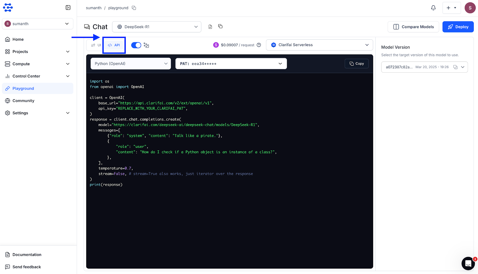
Inside the Playground itself, you may have the choice to view the API part, the place you may entry code snippets in a number of languages, together with cURL, Java, JavaScript, Node.js, the OpenAI-compatible API, the Clarifai Python SDK, PHP, and extra.
You possibly can choose the language you want, copy the snippet, and straight combine it into your functions. For extra particulars on testing fashions and utilizing the Playground, see the Clarifai Playground Quickstart
Attempt it: The Clarifai Playground is the quickest option to check prompts. Navigate to the mannequin web page and click on “Take a look at in Playground”.
By way of the OpenAI‑Appropriate API
Clarifai gives a drop-in alternative for the OpenAI API, permitting you to make use of the identical Python or TypeScript consumer libraries you’re acquainted with whereas pointing to Clarifai’s OpenAI-compatible endpoint. Upon getting your PAT set as an atmosphere variable, you may name any Clarifai-hosted DeepSeek mannequin by specifying the mannequin URL.
Clarifai’s Python SDK simplifies authentication and mannequin calls, permitting you to work together with DeepSeek fashions utilizing concise Python code. After setting your PAT, you may initialize a mannequin consumer and make predictions with only a few strains.
For contemporary net functions, the Vercel AI SDK gives a TypeScript toolkit to work together with Clarifai fashions. It helps the OpenAI-compatible supplier, enabling seamless integration.
{role:“system”,content:“You are a helpful assistant.”},
{role:“user”,content:“What is photosynthesis?”}
],
});
console.log(textual content);
This SDK additionally helps streaming responses, software calling, and different superior options.Along with the above, DeepSeek fashions will also be accessed through cURL, PHP, Java, and different languages. For an entire listing of integration strategies, supported suppliers, and superior utilization examples, discuss with the documentation.
Superior Inference Patterns
DeepSeek fashions on Clarifai assist superior inference options that make them appropriate for production-grade workloads. You possibly can allow streaming for low-latency responses, and software calling to let the mannequin work together dynamically with exterior techniques or APIs. These capabilities work seamlessly via Clarifai’s OpenAI-compatible API.
Streaming Responses
Streaming returns mannequin output token by token, enhancing responsiveness in real-time functions like chat interfaces or dashboards. The instance beneath exhibits the way to stream responses from a DeepSeek mannequin hosted on Clarifai.
importos
fromopenaiimportOpenAI
# Initialize the OpenAI-compatible consumer for Clarifai
Streaming helps you render partial responses as they arrive as an alternative of ready for all the output, lowering perceived latency.
Device Calling
Device calling allows a mannequin to invoke exterior features throughout inference, which is particularly helpful for constructing AI brokers that may work together with APIs, fetch reside information, or carry out dynamic reasoning. DeepSeek-V3.1 helps software calling, permitting your brokers to make context-aware choices. Under is an instance of defining and utilizing a software with a DeepSeek mannequin.
importos
fromopenaiimportOpenAI
# Initialize the OpenAI-compatible consumer for Clarifai
For extra superior inference patterns, together with multi-turn reasoning, structured output technology, and prolonged examples of streaming and power calling, discuss with the documentation
Which DeepSeek Mannequin Ought to I Decide?
Clarifai hosts a number of DeepSeek variants. Selecting the best one relies on your process:
DeepSeek‑R1 – use for reasoning and sophisticated code. It excels at mathematical proofs, algorithm design, debugging and logical inference. Count on slower responses on account of prolonged “pondering mode,” and better token utilization.
DeepSeek‑V3.1 – use for common chat and light-weight coding. V3.1 is a hybrid: it may swap between non‑pondering mode (quicker, cheaper) and pondering mode (deeper reasoning) inside a single mannequin. Superb for summarization, Q&A and on a regular basis assistant duties.
Distilled fashions (R1‑Distill‑Qwen‑7B, and so on.) – these are smaller variations of the bottom fashions, providing decrease latency and value with barely decreased reasoning depth. Use them when pace issues greater than maximal efficiency.
On the time of writing, DeepSeek‑OCR has simply been introduced and isn’t but out there on Clarifai. Regulate Clarifai’s mannequin catalog for updates.
Incessantly Requested Questions (FAQs)
Q1: Do I want a DeepSeek API key? No. When utilizing Clarifai, you solely want a Clarifai Private Entry Token. Don’t use or expose the DeepSeek API key except you’re calling DeepSeek straight (which this information doesn’t cowl).
Q2: How do I swap between fashions in code? Change the mannequin worth to the Clarifai mannequin ID, comparable to openai/deepseek-ai/deepseek-chat/fashions/DeepSeek-R1 for R1 or openai/deepseek-ai/deepseek-chat/fashions/DeepSeek-V3.1 for V3.1.
Q3: What parameters can I tweak? You possibly can alter temperature, top_p and max_tokens to regulate randomness, sampling breadth and output size. For streaming responses, set stream=True. Device calling requires defining a software schema.
This fall: Are there charge limits? Clarifai enforces delicate charge limits per PAT. Implement exponential backoff and keep away from retrying 4XX errors. For prime throughput, contact Clarifai to extend quotas.
Q5: Is my information safe? Clarifai processes requests in safe environments and complies with main information‑safety requirements. Retailer your PAT securely and keep away from together with delicate information in prompts except crucial.
Q6: Can I advantageous‑tune DeepSeek fashions? DeepSeek fashions are MIT‑licensed. Clarifai plans to supply non-public internet hosting and advantageous‑tuning for enterprise prospects within the close to future. Till then, you may obtain and advantageous‑tune the open‑supply fashions by yourself infrastructure.
Conclusion
You now have a quick, normal option to combine DeepSeek fashions, together with R1, V3.1, and distilled variants, into your functions. Clarifai handles all infrastructure, scaling, and orchestration. No separate DeepSeek key or advanced setup is required. Attempt the fashions at present via the Clarifai Playground or API and combine them into your functions.
Pixel 10 Professional Fold customers report battery icon displaying a mysterious query mark.
The bug might be linked to wi-fi chargers, presumably affecting the battery administration system’s calibration.
A brief repair is on the market via a reboot, however Google states {that a} repair will probably be rolled out with the November month-to-month replace.
Google’s newest foldable appears to be dealing with a peculiar bug. A number of Google Pixel 10 Professional Fold customers on Reddit have reported seeing a mysterious query mark(?) as a substitute of the proportion.
This challenge appears to be cropping up for customers who’ve wi-fi chargers, significantly third-party or non-Qi2 licensed chargers, however that is nonetheless hypothesis(as first noticed by Piunika Internet). The rumor on the road is that these chargers may’ve precipitated a “temporary communication or calibration error between the battery administration system and the software program interface, ensuing within the cellphone being uncertain of the present battery stage, therefore the query mark,” the publication added.
Customers on the identical Reddit thread had conflicting opinions on the reason for this glitch. Some say it might be an underlying {hardware} challenge, just like the battery failing, whereas others consider it is a easy UI downside {that a} fast repair may resolve. One consumer even stated that “Lots of this has been occurring because the final play safety replace. I think it can come out as only a bug, however you are good to achieve out to Google to see what they advocate.”
That stated, it is not simply the brand new Pixel 10 Professional Fold dealing with these points; some 9 Professional Fold customers additionally appear to have noticed the bizarre ‘?’ icon subsequent to their battery, the place one consumer said that the error message they acquired was “Unable to learn battery meters”. The consumer appeared to have contacted Google help, who stated they’re sending him a brand new gadget.
(Picture credit score: Nicholas Sutrich / Android Central)
So may this actually be a battery swelling challenge on the brand new Pixel 10 Professional Fold? Solely time will inform. However for now, when you’re seeing this challenge, a short lived repair, all you must do is to reboot the cellphone, which returns the proper battery proportion. In the event you nonetheless do not see it fixing this bug, it’s best to contact Google Help for additional steering or a potential guarantee declare.
Google’s spokesperson additionally confirmed to Android Central that rebooting the gadget will resolve the problem; nevertheless, “Pixel 10 Professional Fold customers ought to use licensed Qi2 wi-fi chargers.” And {that a} repair for this battery bug will probably be rolling out with the November month-to-month replace.
Get the newest information from Android Central, your trusted companion on the planet of Android
Subterranean mosquitoes specialised for all times in subways and sewers first developed to pester people millennia in the past in Mediterranean civilizations.
A broadly accepted story concerning the mosquitoes’ evolution put their origins within the London Underground practice system within the final century or two. However the mosquitoes have really been adapting to humanity’s cities for probably 1000’s of years, researchers report within the Oct. 23 Science.
The northern home mosquito (Culex pipiens) usually bites birds. However one kind present in city underground areas throughout northern latitudes — C. pipiens f. molestus — has developed to feed on people and different mammals. It has key diversifications for dwelling in secluded environments with scarce hosts. The molestus mosquitoes can breed in cramped indoor areas, and when assets are skinny, females can produce eggs with out taking a blood meal.
The mosquitoes have been first acknowledged throughout World Warfare II as they bit Londoners within the Underground in search of refuge from Nazi bombing. The chief speculation was that molestus developed proper there within the Tube. However decades-older historic data of molestus-like mosquitoes within the Mediterranean recommended in any other case, says Yuki Haba, an evolutionary biologist now at Columbia College.
To discover the mosquito’s evolutionary historical past, Haba — then at Princeton College — labored with a global crew of over 200 scientists. The crew compiled, analyzed and in contrast the genomes — the complete set of genetic directions — of 357 home mosquitoes from 77 places throughout western Eurasia.
The molestus lineage far predates the fashionable cities of Europe, the researchers discovered, diverging from their bird-biting cousins between 1,300 and 12,500 years in the past within the Mediterranean and Center East. The mosquitoes might have exploited the irrigation and saved water of early agricultural societies for year-round breeding websites. Adaptation to those settlements might have let the bugs springboard into trendy city environments in a while. Bedbugs took an analogous path to grow to be city pests.
“Adaptation to human areas didn’t want to begin with subways or skyscrapers,” Haba says. “Trendy cities didn’t create molestus — they merely supplied new areas the place its historic, human-associated traits might thrive.”
The mosquitoes’ story has been a textbook instance of recent species arising in response to latest urbanization, says Kristin Winchell, an city evolutionary ecologist at New York College who was not concerned with this analysis.
“All of us simply form of took that as truth, and I believe most of us didn’t notice that it didn’t even have any empirical knowledge backing it up,” she says. “So it’s fairly cool that [the researchers] really got down to check it.”
Lindsay Miles, an city evolutionary biologist at Virginia Tech in Blacksburg, is curious whether or not molestus is interbreeding with aboveground mosquitos across the subway zones the place the trains briefly transfer to aboveground areas. Such hybrids between bird- and human-biting varieties facilitate the unfold of harmful pathogens akin to West Nile virus, which hops from birds to people through the chew of C. pipiens, Haba says.
Future work might reveal how the mosquitoes are nonetheless evolving, says research coauthor Lindy McBride, an evolutionary biologist at Princeton College. “Despite the fact that they didn’t originate in cellars and subways, they’re there now and are most probably within the means of adapting additional to this distinctive surroundings.”
The target market for immediately’s submit is future-me, and anybody else equally within the fairly particular points it’s jotting down notes for. These points embrace:
Drawing directed graphs with ggdag which have totally different colored edges
Accessing the UN Sustainable Improvement Objectives (SDGs) database API
Information choices on gender inequality
Becoming the identical blended results mannequin with lme4::lmer, mgcv::gamm and mgcv::gam, evaluating outcomes and extracting group-level residuals
Hand-drawing prediction plots to indicate the outcomes of fashions with interactions and evaluating that to the marginaleffects package deal
Diagnostics of a simplified model of the mannequin
Modelling technique questions regarding researcher levels of freedom, use of splines and interplay results
My method to presenting this (each immediately, and in Half I) is totally different to my standard one, the place I attempt to make the submit itself a stand-alone, reproducible artefact with all of the code essential to provide the leads to the submit. That method simply didn’t work out on this case; the code was too lengthy and boring to incorporate in the principle weblog, there are too many various audiences to write down for, and I went down too many useless ends in exploring a few of the modelling choices. Even on this technical companion piece, this submit isn’t going to be totally reproducible, however simply have the snippets of code that greatest illustrate the purpose.
Directed graphs with totally different colored edges
For the principle submit, I had to attract a few directed graphs with totally different colored edges connecting the nodes. Particularly, I wished to make use of a crimson line to indicate a destructive route impact, and blue to indicate a constructive, like this:
This was surprisingly fiddly to do and required a little bit of a hack. Particularly, you must explicitly name the tidy_dagitty operate, which turns a ggdag graph object of sophistication dagitty into an information body of sophistication tidy_dagitty; then you definitely add a column to that knowledge body which has the precise colors as its values, conditional on no matter algorithm it’s good to decide these colors. On this instance, I need it to be crimson when the road phase is join “opp” (Alternatives for girls and women) to “tfr” (Complete fertility fee), and blue in any other case.
So far as I might inform, you possibly can’t simply map a column of character or issue values to color and let the color scale match it, which might be the method extra according to the ggplot2 philosophy. As an alternative, you solely have the selection of an identification scale, which is why that column edge_type I add has to have the values “darkred” and “steelblue”. That’s the principle trick for doing this.
dg2<-dagify(tfr~opp+hw,hw~opp,labels=c("tfr"="Complete fertility fee","hw"="Males doing home tasks","opp"="Alternatives fornwomen and women"),consequence="tfr",publicity="hw")|># explicitly name this often hidden operate so we are able to color the sides:ggdag::tidy_dagitty(seed=124)|># color the sides. Have to specify identification of color right here, not use scale_mutate(edge_type=ifelse(to=="tfr"&title=="opp","darkred","steelblue"))# Draw the simplified causal graphset.seed(124)dg2|>ggplot(aes(x=x,y=y,xend=xend,yend=yend))+geom_dag_node(color="gray")+geom_dag_edges(aes(edge_colour=edge_type),arrow_directed=grid::arrow(size=unit(12,"pt"),sort="closed"))+geom_dag_text_repel(aes(label=label),col=lab_col)+theme_dag(base_family="Roboto")
Accessing the UN SDGs database
I couldn’t discover a easy manner of accessing the United Nations Statistics Division’s invaluable definitive database of the SDG indicators for all nations of the world. By which I imply, it has an API, however I didn’t see anybody who’d written a pleasant R package deal to conveniently work together with it. If anybody is aware of of somebody who’s finished this, or needs to do it themselves, please let me know.
So I needed to write my very own API request on my own, like an animal. I did this in what I’m positive is a suboptimal manner, but it surely works. From taking part in round with the UN’s API I discovered the curl command I wished to obtain the info:
Then I used features from Bob Rudis’ curlconverter R package deal to transform this to a request for the old style httr package deal to make use of. Because the feedback on this code say, I do know all that is outmoded; but it surely works for now.
#-----------downloading some SDG time use knowledge from the UN database-------------# Be aware positive that is the easiest way to do that, it was clunky to work out,# but it surely works. Somebody ought to (or have they already?) construct an R package deal.## that is all httr, I perceive httr2 is the present factor now, however this nonetheless works library(curlconverter)library(httr)request<-"curl -X POST --header 'Content material-Kind: utility/x-www-form-urlencoded' --header 'Settle for: utility/octet-stream' -d 'seriesCodes=SL_DOM_TSPD' 'https://unstats.un.org/sdgapi/v1/sdg/Collection/DataCSV'"|>straighten()|>make_req()gender_txt<-content material(request[[1]](),as="textual content")gender<-read_csv(gender_txt)|>clean_names()
The tip outcomes is I desire a variable, from that SL_DOM_TPSD indicator (time spent on home chores and care work by intercourse and concrete/rural location) that may be represented like this:
There are vital knowledge wrangling challenges, although, particularly the totally different age classes utilized in every nation, the totally different years that surveys had been carried out, and the presence of a number of observations for some however not all nations.
The primary motive for together with this subsequent snippet is to remind myself of what was wanted to do to fiddle with these age classes. For instance, notice that some nations have values for a number of open ended classes like 3+ and 15+; we want a rule for deciding which of those is greatest for our desired constructed variable of males’s share of grownup home home and care work (on this case, 15+ is best than 3+, when each can be found for a rustic):
rely(gender,intercourse)# two classes, FEMALE and MALE - no TOTALrely(gender,age)# many various ages used for various nationsrely(gender,location)# there's ALLAREA, RURAL and URBAN# needs to be just one indicator:stopifnot(size(distinctive(gender$series_description))==1)# which is # Proportion of time spent on unpaid home chores and care work, by intercourse, age and placement (%) time_chores<-gender|># we do not need rural and concrete, simply nation complete:filter(location=="ALLAREA")|># we wish the ages like 15+, 12+ and so on, not these like 15-59 with an higher certainfilter(grepl("^[0-9]*+$",age))|># however not the retirees, which some nations embrace. We wish the 15+, not 15+# and 65+ individually:filter(!age%in%c("65+","85+","60+"))|># calculate the male time spent as a proportion of complete (female and male) time spentgroup_by(geo_area_name,time_period,age)|>summarise(prop_male=worth[sex=='MALE']/sum(worth[sex=='MALE']+worth[sex=='FEMALE']))|>group_by(geo_area_name)|># Label the most recent survey per nation. Be aware that any modelling must# embrace a rustic random impact for the a number of observations per nation:mutate(is_latest=ifelse(time_period==max(time_period),"Most up-to-date","Earlier"))|># restrict to only the most effective age group, closest to adults, for every nation/time:group_by(geo_area_name,time_period)|>mutate(age=issue(age,ranges=c("15+","16+","18+","12+","10+","6+","5+","3+")))|>prepare(geo_area_name,time_period,age)|>slice(1)|>ungroup()|>mutate(iso3_code=countrycode(geo_area_name,origin="nation.title.en",vacation spot="iso3c"))
Information on gender inequality
I spent fairly a little bit of time on the lookout for knowledge on gender inequality unbiased of the home tasks query. I wished one thing that resembled ladies’s and women’ alternatives in training and the financial system extra broadly. I had varied deadends in pursuing this. My first concept was some type of literacy measure—feminine literacy at some given age, or for adults total, as a ratio for equal male literacy. However the varied sources for this simply didn’t have sufficient observations.
The primary sources for literacy can be self-report in a census or presumably a social survey; or a standardised check at a given yr of education. After some fruitless time with SDGs, the World Financial institution’s World Improvement Indicators, and varied different sources, I concluded that neither of those appear to be available in a comparable foundation for sufficient years that matched with the year-country mixtures that I had time-use knowledge for.
I ended up utilizing the Gender Inequality Index (GII) from the UNDP as an alternative. Now, this index is advanced and depends on a bunch of indicators which might be clearly going to be at the very least as laborious to measure as literacy—like degree of secondary training (wants admin knowledge or survey or census) and maternal mortality ratio (wants good civil registry, or survey knowledge as a much less passable different). Right here’s how the GII is constructed:
However the GII is offered for all country-year mixtures, which merely can’t be based mostly on direct observations of those variables. Clearly the UNDP do a bunch of modelling to interpolate all of the lacking values. I didn’t look into this however simply trusted the UNDP to have finished the most effective job attainable. It’s definitely very handy to get this measure of gender inequality for thus many nations (206 ‘nations’, however this contains some regional groupings), and for thus a few years.
There have been a number of methods to obtain this GII knowledge from the Human Improvement Experiences web site, but it surely seems the most effective is to obtain all of the Human Improvement Report knowledge for the most recent yr in a single, massive CSV:
# You'll be able to obtain all of the HDR elements (together with GII):df<-"hdr25.csv"if(!file.exists(df)){obtain.file("https://hdr.undp.org/websites/default/information/2025_HDR/HDR25_Composite_indices_complete_time_series.csv",destfile=df)}hdr<-read_csv(df)
From there it’s simple knowledge wrangling to extract simply the GII knowledge and mix with my different datasets utilizing yr and the ISO three character codes for nations to affix by.
Becoming the identical blended results mannequin with lmer, gamm and gam
Specifying fashions
One of many issues I wished to kind on this submit was the close to equivalence of a few of the many various methods of specifying and becoming a blended results mannequin in R. There’s an excellent submit from Gavin Simpson on ‘Utilizing random results in GAMs with mgcv’ that I referred to repeatedly in making ready this.
Particularly, I wished to verify that these 4 fashions, set out under, are all very comparable. By which I truly imply the final three are equivalent statistically, however have other ways of being estimated and/or the components written down; and the primary is a statistically totally different mannequin when it comes to chance distributions and hyperlink features, however successfully very very comparable certainly to the opposite three:
# notice response variable is ltfr, outlined earlier as log(tfr):model2<-lmer(ltfr~gii+log(gdprppppc)*prop_male+(1|country_fac),knowledge=model_ready)model7a<-gamm(tfr~gii+log(gdprppppc)*prop_male+s(country_fac,bs='re'),knowledge=model_ready,household=quasipoisson)model7b<-gamm(tfr~gii+log(gdprppppc)*prop_male,random=checklist(country_fac=~1),knowledge=model_ready,household=quasipoisson)model7c<-gam(tfr~gii+log(gdprppppc)*prop_male+s(country_fac,bs='re'),knowledge=model_ready,household=quasipoisson,technique="REML")
These are:
model2 – match with lme4::lmer, response variable is log-transformed first after which response is Gaussian, nation degree random impact is specified with 1 | country_fac components notation. Be aware that I can’t use glmer becuase it doesn’t enable household = quasipoisson.
model7a – match with mgcv::gamm which is an iterative course of the place the blended results are with with lmer and smoothing splines are finished with gam, iterate until converges. The tip end result incorporates the ultimate model of each the lme mannequin and the gam mannequin. There’s no pre-transformation finished of the response variable as a result of we’re utilizing a generalized linear mannequin with quasipoisson household – that’s, variance is proportional to the imply, however not compelled to be equal to it. The random nation degree impact is specified with s(country_fac, bs="re") (re stands for random results), which is handed on to lme that treats it as Formulation: ~1 | country_fac.
model7b – equivalent to 7a besides the random results are specified by random = checklist(country_fac = ~ 1)
model7c – match with mgcv::gam, utilizing the identical mannequin specification as model7b. In contrast to gamm, this does all of the work inside gam itself, there’s no iterating to the features of the lme4 package deal. There are limitations imposed consequently – the random results can’t be correlated with eachother, and you’ll’t specify advanced error buildings (autocorrelation and so on) like you might with gamm or lmer. However I don’t have a necessity for both of this stuff. Importantlymodel7c has to make use of restricted most probability as its estimation technique if we wish it to get equal outcomes to the lmer-based strategies.
Ultimately, none of those fashions had been referred to in my essential submit as a result of I went for an method based mostly purely on the usage of gam() and with varied non-linear results even within the base, null mannequin. Nevertheless it was a really helpful studying expertise for me to work out precisely what’s and isn’t totally different in a bunch of comparable mannequin specs.
Getting the identical fastened coefficients
Right here is code to extract the coefficients for the fastened results from these 4 basically equivalent fashions:
# Mounted coefficients of the 4 comparable linear fashions:abstract(model7a$lme)$tTable|>as.knowledge.body()|>choose(mod7a=Worth)|>mutate(mod7b=pull(as.knowledge.body(abstract(model7b$lme)$tTable),Worth))|>mutate(mod7c=pull(as.knowledge.body(abstract(model7c)$p.desk),Estimate))|>mutate(mod2=fixef(model2))|>mutate(throughout(the place(is.numeric),spherical,digits=2))
The largest distinction within the coefficients is with model2, not shocking as a result of it has the largest distinction in its specification from the opposite three. The log transformation is finished earlier than modelling and the response is then handled as Gaussian, versus the quasipoisson hyperlink and variance features method of the opposite three.
Be aware that from the above snippet of code that not least of the variations between these fashions is the totally different strategies used to extract these fastened coefficients.
Getting the identical group degree random results
One other verify that these fashions are principally the identical was to check the country-level random results. For instance, is the “Oman” impact going to be the identical in every of those 4 fashions?
To reply this I first needed to work out the right way to extract the random results from the variations that used the s(country_fac, bs="re") notation to set the random results. It seems the easiest way to do that is with the gratia package deal by Gavin Simpson (once more), which has the smooth_coefs operate for this and associated functions. So this subsequent chunk of code extracts all these nation results and attracts a pairs plot of them.
Which provides this end result, with a satisfying excessive correlation within the nation results of the 4 totally different fashions:
Once more, model2 is a bit totally different from the opposite three, for a similar motive. I’m truly struck with how a lot we get near-identical leads to a mannequin that does the log transformation earlier than modelling to those who use a log hyperlink operate.
Displaying marginal results
In some unspecified time in the future when taking part in round with the other ways of specifying fashions I used to be having bother understanding a few of the output—some coefficients I assumed needs to be equivalent weren’t—and began constructing my very own, very primary predicted imply values, by multiplying numbers by the coefficients. The unique drawback went away after I found some mistake or different, however I repurposed what I’d finished into the code to provide this plot.
That is the form of plot I’d been imagining to make use of for instance the interplay of the male home tasks variable with GDP per capita. I’d been anticipating to see one thing like this as soon as I’d seen the route of the development swap round in excessive revenue nations in comparison with low revenue nations:
This plot was produced with this very hacked-together, brittle, operate that multiplies variables by their coefficients:
# Handbook manner of constructing a plot. Not even utilizing predict()b<-fixef(model2)#' Predict TFR given these coefficientscalc_tfr<-operate(prop_male,gdp,gii=imply(model_ready$gii)){exp(b[1]+b[2]*gii+b[3]*log(gdp)+b[4]*prop_male+b[5]*prop_male*log(gdp))}# Dwelling-made prediction plot to indicate the interplay impact:tibble(prop_male=rep(seq(from=0.05,to=0.45,size.out=50),3),gdp=rep(c(3000,10000,80000),every=50))|>mutate(tfr=c(calc_tfr(prop_male,gdp)),gdp=greenback(gdp),gdp=fct_relevel(gdp,"$3,000"))|>ggplot(aes(x=prop_male,color=gdp,y=tfr))+geom_line(linewidth=1.5)+geom_point(knowledge=model_ready,color="black")+scale_x_continuous(label=%)+labs(x="Proportion of grownup home tasks finished by males",y="Predicted complete fertility fee",title="Interplay of revenue, home tasks finished by males on fertility fee",subtitle="Calculations finished for a hypothetical nation that in any other case has the common Gender Inequality Index",color="PPP GDP per capita",caption=full_caption)
It’s not one thing I’d use for actual as a result of I’d need to calculate the usual errors at every level too. In some unspecified time in the future, we are saying that’s what the varied package deal authors gave us the predict technique for the lessons they made holding fitted fashions. However even utilizing predict and making use of it to a rigorously chosen grid of values is made simple nowadays by the marginaleffects package deal, by Vincent Arel-Bundock, Noah Greifer and Andrew Heiss. I used to be utilizing this for the primary critical time on this train.
It seems that marginaleffects is nice for this function; simple to make use of to get you an almost adequate plot. Right here’s the outcomes of the marginaleffects::predict_plot()
It’s like my home-made plot, however higher in at the very least one respect; it has confidence intervals. There have been some hitches in scales and guides:
the y axis actually wished to be labelled on the dimensions of the linear predictor, and ultimately I let it have its manner and add a secondardy axis on the proper hand aspect labelled on the unique scale
controling the color scale non-trivial, as did labelling it with $ indicators. Ultimately I didn’t persist on this; there are methods to get plot_predictions to provide the knowledge fairly than draw a plot, however I didn’t sluggish issues down.
Right here’s the good and easy code to attract that; the “good and easy” bit partiuclarly referring to the straightforward manner you possibly can specify the variables’ values for instance. As soon as I’d realised how simple this was, I used it for the remainder of the weblog submit, together with the significantly extra advanced generalized additive fashions that had been my precise most popular fashions.
plot_predictions(model2,factors=1,situation=checklist("prop_male","gdprppppc"=c(3000,10000,80000)))+scale_y_continuous(trans=transform_exp(),breaks=log(c(2,4,6)),label=comma,sec.axis=sec_axis(exp,title="Complete Fertility Fee"))+scale_x_continuous(label=%)+labs(y="log(complete fertility fee)",color="PPP GDP per capita",fill="PPP GDP per capita",x="Proportion of grownup home tasks finished by males",title="Interplay of revenue, home tasks finished by males on fertility fee",subtitle="Calculations finished for a hypothetical nation that in any other case has the common Gender Inequality Index",caption=full_caption)# notice the warning that this solely takes into consideration the uncertainty of# fixed-effect parameters. That is in all probability okay? if we're all for # the causality fairly than predicting new nations?
Modelling selections and checks
Detoured into the backyard of forking paths?
Now, all that stuff within the earlier part is usually cosmetics. Eager readers could have observed that the mannequin described there may be not the one I utilized in the principle weblog in any respect. Specifically, it has a simple linear interplay of GDP per capita and male home tasks, whereas I in the end used a smoothed spline interplay as an alternative; I added a smoothed time impact; and made gender inequality index additionally a non-linear spline.
To refresh reminiscences, the 2 fashions contrasted in the principle weblog had been these two:
I discovered model6b defined just about no additional deviance in comparison with model4b. The distinction between model6b and the model2 used above is all of the s() splines, and the nuisance impact of time_period being managed for.
In case you have a look at the plot within the earlier part displaying the marginal impact of elevated male home work from the linear mannequin with no splines, it seems to be vital. And the output appears to substantiate this—the abstract under reveals the male home work as negatively associated to fertility, and its interplay with GDP per capita as positively associated (so for increased GDP per capita AND increased ranges of male home tasks, complete fertility fee goes up). These are clearly vital at typical ranges. And that is the other of what I reported in my weblog, which was that there was no male home tasks affect on fertility after we management for gender inequality and GDP per capita.
> abstract(model2, cor = FALSE)
Linear blended mannequin match by REML ['lmerMod']
Formulation: ltfr ~ gii + log(gdprppppc) * prop_male + (1 | country_fac)
   Information: model_ready

REML criterion at convergence: -149.8

Scaled residuals:
     Min       1Q   Median       3Q      Max
-3.03513 -0.41571  0.07449  0.46057  2.51483

Random results:
 Teams      Title        Variance Std.Dev.
 country_fac (Intercept) 0.037475 0.1936
 Residual                0.008724 0.0934
Variety of obs: 172, teams:  country_fac, 79

Mounted results:
                         Estimate Std. Error t worth
(Intercept)               3.65360    0.60667   6.022
gii                       1.26916    0.20080   6.320
log(gdprppppc)           -0.34957    0.06275  -5.571
prop_male                -8.51667    2.05957  -4.135
log(gdprppppc):prop_male  0.90124    0.21501   4.192
That is the place I come to an issue that truly worries me—did I am going down the backyard of forking paths? You might accuse me of constructing the mannequin extra advanced—by including a time impact, non-linear gender inequality impact and GDP per capita results—till I obtained the specified end result, of no remaining deviance defined by male time spent on home tasks.
My defence towards this must be that I at all times meant so as to add in these non-linear results, and that I’d solely stopped to specify these fashions with out them as a result of I wished to take a look at the lmer v gam v gamm specification query. And that is true. Nevertheless it’s additionally true that I had anticipated that even with out non-linear splines added, the male time on home tasks can be non-significant; an expectation that turned out to be mistaken.
The truth is, earlier than happening the lmer v gam v gamm rabbit gap, I had began with a model0, specified by this:
# A primary null mannequin:model0<-lmer(ltfr~gii+log(gdprppppc)+(1|country_fac),knowledge=model_ready)
I had then finished this diagnostic verify, and a plot of the residual fertility fee towards male home tasks (backside proper panel within the plot under):
This appeared (visually) like solely random noise remained, and I in all probability obtained careless in assuming that splines and stuff, whereas the place I wished to move, weren’t important, therefore it was okay to suit these linear fashions first. It’s simply that when it turned out that there was an obvious “vital” impact from doing this, I used to be left with a grimy style in my mouth that I used to be attempting becoming fashions till I discovered the one which suited my expectation (of no male home tasks impact after controlling for gender inequality and GDP per capita).
Fortunately, that is solely a weblog; no-one expects me to pre-register my analytical plan for it; and anyway I’m satisfied of the substance of the ultimate discovering; and I actually do bear in mind intending to make use of the variations with splines. However I’m guessing lots of researchers really feel this once they train their researcher levels of freedom.
Spline v tensor product smooths
Once I posted the principle weblog, Stephen Wild made the next remark: “I’m interested in s(log(gdprppppc), prop_male) in your mannequin fairly than ti(log(gdprppppc), prop_male)”. The truth is, I hadn’t thought-about this feature, and I ought to have. So after this remark I went again and match a brand new mannequin with tensor product smooths. Be aware that it’s additionally essential so as to add the ti(prop_male) + ti(log(gdprppppc) single phrases explicitly on this case, not like when utilizing s().
That manner of specifying the person phrases with eg ti(prop_male) isn’t a kind of urged by Gavin Simpson right here; I believe it’s okay although. If not I’ll likely have a future weblog attempting to get this straight in my head.
Now, ideally I might have a digression right here the place I clarify the theoretical and sensible variations between spline and tensor product smooths and when to make use of every, however I’m not feeling as much as that. One factor I do know is {that a} tensor product clean is invariant to modifications within the authentic scale of the variable, which might make it extra strong in case you’re involved about totally different scales of your totally different variables; this appears to me the principle level emphasised when this concern is mentioned in Gavin Simpson’s definitive ebook on generalized additive fashions in R
Anyway, on this specific case there’s little to selected from, as seen on this thrown collectively assortment of plots. These within the high present the GDP per capita and male home tasks results when utilizing a tensor product clean; these on the backside are the identical when utilizing a spline:
My hunch is that the tensor product clean is a bit higher right here, however I received’t change historical past by modifying the principle weblog to make use of it. The addition of the male_prop variable nonetheless isn’t statistically ‘vital’; whereas we are able to see that for increased revenue nations there’s a little bit of an upwards slope (within the high proper panel of the gathering of plots above), it’s not explaining a fabric quantity of additional materials.
There’s negligible additional deviance defined by the mannequin with the prop_male and its GDP interplay, in comparison with the easier mannequin with out them.
Truly, I don’t actually have a lot so as to add right here.
I might have talked extra about a few of this, eg that unexplained okay=3 within the spline for gender inequality, and my interested by diagnostic plots for GAMs (and my rushed, imperfect implementation of it); however in some unspecified time in the future there are diminishing marginal returns. I’ve coated off the principle issues right here; largely issues that I believe future-me will need to consult with subsequent time I’m doing comparable issues.
For some individuals, it’s in all probability value testing the full script of authentic code if there’s further factors of curiosity or questions.