Thursday, February 12, 2026
Home Blog Page 24

7 Below-the-Radar Python Libraries for Scalable Characteristic Engineering


7 Below-the-Radar Python Libraries for Scalable Characteristic Engineering
Picture by Editor


Introduction

 
Characteristic engineering is an important course of in information science and machine studying workflows, in addition to in any AI system as a complete. It entails the development of significant explanatory variables from uncooked — and infrequently somewhat messy — information. The processes behind characteristic engineering might be very simple or overly complicated, relying on the amount, construction, and heterogeneity of the dataset(s) in addition to the machine studying modeling targets. Whereas the preferred Python libraries for information manipulation and modeling, like Pandas and scikit-learn, allow fundamental and reasonably scalable characteristic engineering to some extent, there are specialised libraries that go the additional mile in coping with large datasets and automating complicated transformations, but they’re largely unknown to many.

This text lists 7 under-the-radar Python libraries that push the boundaries of characteristic engineering processes at scale.


1. Accelerating with NVTabular

 
First up, we now have NVIDIA-Merlin’s NVTabular: a library designed to use preprocessing and have engineering to datasets which are — sure, you guessed it! — tabular. Its distinctive attribute is its GPU-accelerated method formulated to simply manipulate very large-scale datasets wanted to coach huge deep studying fashions. The library has been significantly designed to assist scale pipelines for contemporary recommender system engines based mostly on deep neural networks (DNNs).


2. Automating with FeatureTools

 
FeatureTools, designed by Alteryx, focuses on leveraging automation in characteristic engineering processes. This library applies deep characteristic synthesis (DFS), an algorithm that creates new, “deep” options upon analyzing relationships mathematically. The library can be utilized on each relational and time collection information, making it potential in each of them to yield complicated characteristic era with minimal coding burden.

This code excerpt exhibits an instance of what making use of DFS with the featuretools library seems to be like, on a dataset of consumers:

customers_df = pd.DataFrame({'customer_id': [101, 102]})
es = es.add_dataframe(
    dataframe_name="prospects",
    dataframe=customers_df,
    index="customer_id"
)

es = es.add_relationship(
    parent_dataframe_name="prospects",
    parent_column_name="customer_id",
    child_dataframe_name="transactions",
    child_column_name="customer_id"
)


3. Parallelizing with Dask

 
Dask is rising its recognition as a library to make parallel Python computations quicker and less complicated. The grasp recipe behind Dask is to scale conventional Pandas and scikit-learn characteristic transformations by way of cluster-based computations, thereby facilitating quicker and inexpensive characteristic engineering pipelines on massive datasets that might in any other case exhaust reminiscence.

This article exhibits a sensible Dask walkthrough to carry out information preprocessing.


4. Optimizing with Polars

 
Rivalling with Dask by way of rising recognition, and with Pandas to aspire to a spot on the Python information science podium, we now have Polars: a Rust-based dataframe library that makes use of lazy expression API and lazy computations to drive environment friendly, scalable characteristic engineering and transformations on very massive datasets. Deemed by many as Pandas’ high-performance counterpart, Polars could be very straightforward to study and familiarize with in case you are pretty conversant in Pandas.

to know extra about Polars? This article showcases a number of sensible Polars one-liners for frequent information science duties, together with characteristic engineering.


5. Storing with Feast

 
Feast is an open-source library conceived as a characteristic retailer, serving to ship structured information sources to production-level or production-ready AI functions at scale, particularly these based mostly on massive language fashions (LLMs), each for mannequin coaching and inference duties. One in all its enticing properties consists of making certain consistency between each levels: coaching and inference in manufacturing. Its use as a characteristic retailer has turn out to be carefully tied to characteristic engineering processes as nicely, specifically by utilizing it together with different open-source frameworks, for example, denormalized.


6. Extracting with tsfresh

 
Shifting the main focus towards massive time collection datasets, we now have the tsfresh library, with a bundle that focuses on scalable characteristic extraction. Starting from statistical to spectral properties, this library is able to computing as much as a whole bunch of significant options upon massive time collection, in addition to making use of relevance filtering, which entails, as its identify suggests, filtering options by relevance within the machine studying modeling course of.

This instance code excerpt takes a DataFrame containing a time collection dataset that has been beforehand rolled into home windows, and applies tsfresh characteristic extraction on it:


features_rolled = extract_features(
    rolled_df, 
    column_id='id', 
    column_sort="time", 
    default_fc_parameters=settings,
    n_jobs=0
)


7. Streamlining with River

 
Let’s end dipping our toes into the river stream (pun meant), with the River library, designed to streamline on-line machine studying workflows. As a part of its suite of functionalities, it has the aptitude to allow on-line or streaming characteristic transformation and have studying methods. This will help effectively take care of points like unbounded information and idea drift in manufacturing. River is constructed to robustly deal with points hardly ever occurring in batch machine studying techniques, resembling the looks and disappearance of information options over time.


Wrapping Up

 
This text has listed 7 notable Python libraries that may assist make characteristic engineering processes extra scalable. A few of them are straight targeted on offering distinctive characteristic engineering approaches, whereas others can be utilized to additional assist characteristic engineering duties in sure eventualities, together with different frameworks.


Iván Palomares Carrascosa is a frontrunner, author, speaker, and adviser in AI, machine studying, deep studying & LLMs. He trains and guides others in harnessing AI in the true world.

Apple simply fully modified how you purchase a Mac

0

‘Again to the Moon’: Time journal salutes Artemis 2 astronauts in particular commemorative cowl concern

0


Perched on Kennedy Area Heart’s Launch Pad 39B, NASA’s Artemis 2 SLS rocket is poised to propel itself into the heavens as early as Feb. 8, for a 10-day lunar flyby mission carrying astronauts Reid Wiseman, Jeremy Hansen, Victor Glover and Christina Koch of their Orion spacecraft.

Whereas the world holds its collective breath and awaits humanity’s return to the moon after greater than a half-century for a record-breaking lunar voyage, Time journal is celebrating the momentous occasion with a particular Artemis 2 cowl concern that hit newsstands on Friday (Jan. 30).

The Artemis 2 crew lands on the brand new cowl of Time journal. (Picture credit score: Time Journal)

Kluger’s predominant Artemis 2 characteristic, entitled “Again to the Moon,” delivers participating context and offers contrasts and comparisons to Apollo 8. That 1968 NASA mission was the primary crewed flight to orbit the moon and return safely, and helped pave the best way for Apollo 11‘s lunar touchdown in July 1969. The significance of that first flight past Earth orbit cannot be overstated, because the destiny of the whole program relied on the success of its crew of Jim Lovell, Frank Boorman and William Anders.

ARMA processes with nonnormal disturbances

0


Autoregressive (AR) and moving-average (MA) fashions are mixed to acquire ARMA fashions. The parameters of an ARMA mannequin are usually estimated by maximizing a chance operate assuming independently and identically distributed Gaussian errors. It is a reasonably strict assumption. If the underlying distribution of the error is nonnormal, does most chance estimation nonetheless work? The quick reply is sure beneath sure regularity circumstances and the estimator is named the quasi-maximum chance estimator (QMLE) (White 1982).

On this put up, I exploit Monte Carlo Simulations (MCS) to confirm that the QMLE of a stationary and invertible ARMA mannequin is constant and asymptotically regular. See Yao and Brockwell (2006) for a proper proof. For an outline of performing MCS in Stata, discuss with Monte Carlo simulations utilizing Stata. Additionally see A simulation-based clarification of consistency and asymptotic normality for a dialogue of performing such an train in Stata.

Simulation

Let’s start by simulating from a stationary and invertible ARMA(1,1) course of:
[
y_t = 0.8 y_{t-1} + epsilon_t + 0.5 epsilon_{t-1}
]

I assume a demeaned (chi^2(1)) distribution for (epsilon_t). The next code implements an MCS for the parameters of an ARMA(1,1) course of with demeaned chi-squared improvements. At every repetition, I’ll draw from the method, estimate the parameters of the method, and carry out Wald checks with null hypotheses that correspond to the true parameter values.


. clear all

. set seed 2016

. native MC = 5000

. native T = 100

. quietly postfile armasim ar_t100 ma_t100 rr_ar_t100 rr_ma_t100 utilizing t100, 
> exchange

. forvalues i=1/`MC' {
  2.         quietly drop _all
  3.         native obs = `T' + 100
  4.         quietly set obs `obs'
  5.         quietly generate time = _n
  6.         quietly tsset time
  7. /*Generate information*/
.         quietly generate eps = rchi2(1)-1
  8.         quietly generate y = rnormal(0,1) in 1
  9.         quietly exchange y = 0.8*l.y + eps + 0.5*l.eps in 2/l
 10.         quietly drop in 1/100
 11. /*Estimate*/
.         quietly arima y, ar(1) ma(1) nocons vce(sturdy)
 12.         quietly take a look at _b[ARMA:l.ar]=0.8
 13.         native r_ar = (r(p)<0.05)
 14.         quietly take a look at _b[ARMA:l.ma]=0.5
 15.         native r_ma = (r(p)<0.05)
 16.         put up armasim (_b[ARMA:l.ar]) (_b[ARMA:l.ma]) (`r_ar') (`r_ma')
 17. }

. postclose armasim

Traces 1–2 clear Stata and set the seed of the random quantity generator. Traces 3–4 assign the variety of Monte Carlo repetitions and the pattern measurement to native macros MC and T, respectively. Right here I’ll carry out 5,000 Monte Carlo repetitions with a pattern measurement of 100.

In line 5, I exploit postfile to create a spot in reminiscence referred to as armasim to retailer simulation outcomes. We are going to retailer the AR and MA estimates of the ARMA(1,1) mannequin from every Monte Carlo repetition. The outcomes of the Wald checks for the AR and MA parameters will even be saved. These binary variables maintain the worth 1 if the null speculation is rejected on the 5% stage. Every variable is suffixed with the pattern measurement, and can be saved within the dataset t100.

I exploit forvalues to carry out the Monte Carlo repetitions. Every time by the forvalues loop, I begin by dropping all variables and setting the variety of observations to the pattern measurement plus 100. These first 100 observations can be discarded as burn-in. I then generate a time variable and declare it as time-series information.

Subsequent, I generate information from an ARMA(1,1) course of. First, I draw demeaned (chi^2(1)) improvements and retailer them within the variable eps. I retailer the noticed collection in y. The burn-in observations are then dropped.

I estimate the parameters of the ARMA(1,1) mannequin utilizing the arima command, which on this case needs to be interpreted as a QMLE. Notice that I specify nocons to suppress the fixed time period. I exploit vce(sturdy) to request customary errors sturdy to misspecification as a result of the default customary errors are primarily based on a traditional distribution and are invalid on this case. I take a look at whether or not the parameters are equal to their true values and use the put up command to retailer the estimates together with the rejection charges of the Wald checks in armasim.

After the forvalues loop, I shut armasim in reminiscence utilizing postclose. This protects all of the estimates within the dataset t100.

I’ve demonstrated the best way to carry out a Monte Carlo simulation with 5,000 repetitions of an ARMA(1,1) course of with a pattern measurement of 100. I repeat the identical experiment for a pattern measurement of 1,000 and 10,000 and retailer the estimates within the datasets t1000 and t10000, respectively. The code is supplied within the Appendix.

Now, I consider the outcomes of the simulations for the QMLE of the AR parameter. The identical strategies can be utilized to judge the estimator for the MA parameter.

Consistency

A constant estimator will get arbitrarily shut in likelihood to the true worth as you enhance the pattern measurement. I’ll assess the consistency of the QMLE for the AR parameter by evaluating the outcomes of our three simulations.

I load the t100 information in reminiscence and merge with the t1000 and t10000 datasets utilizing the merge command. Then I plot the empirical densities of the estimated AR parameter for the three pattern sizes.


. use t100, clear

. quietly merge 1:1 _n utilizing t1000

. drop _merge

. quietly merge 1:1 _n utilizing t10000

. drop _merge

. kdensity ar_t100, n(5000) generate(x_100 f_100) kernel(gaussian) nograph

. label variable f_100 "N=100"

. kdensity ar_t1000, n(5000) generate(x_1000 f_1000) kernel(gaussian) nograph

. label variable f_1000 "N=1000"

. kdensity ar_t10000, n(5000) generate(x_10000 f_10000) kernel(gaussian) 
> nograph

. label variable f_10000 "N=10000"

. graph twoway (line f_100 x_100) (line f_1000 x_1000) (line f_10000 x_10000),
> legend(rows(1)) title("Empirical densities") subtitle("Autoregressive paramet
> er")

The empirical distribution for the estimated AR parameter is tighter across the true worth of 0.8 for a pattern measurement of 10,000 than that for a pattern of measurement 100. The determine implies that as we preserve rising the pattern measurement to (infty), the AR estimate converges to the true worth with likelihood 1. This means that the QMLE is constant.

Asymptotic normality

If (hat{theta}_{textrm{QMLE}}) is a constant estimator of the true worth (theta), then (sqrt{T}(hat{theta}_{textrm{QMLE}}-theta)) converges in distribution to (N(0,V)) as (T) approaches (infty) (White 1982). Assuming I’ve an infinite variety of observations, the sturdy variance estimator offers a very good approximation to the true variance. On this case, I get hold of the “true” variance for the recentered and rescaled AR parameter to be 0.42 by utilizing the sturdy variance estimator on a 10-million statement pattern.

Let us take a look at the recentered and rescaled model of the empirical distributions of the AR parameters obtained for various pattern sizes. I plot all of the empirical distributions together with the “true” N(0,0.42) distribution for comparability.


. generate double ar_t100n = sqrt(100)*(ar_t100 - 0.8)

. generate double ar_t1000n = sqrt(1000)*(ar_t1000 - 0.8)

. generate double ar_t10000n = sqrt(10000)*(ar_t10000 - 0.8)

. kdensity ar_t100n, n(5000) generate(x_100n f_100n) kernel(gaussian) nograph

. label variable f_100n "N=100"

. kdensity ar_t1000n, n(5000) generate(x_1000n f_1000n) kernel(gaussian) 
> nograph

. label variable f_1000n "N=1000"

. kdensity ar_t10000n, n(5000) generate(x_10000n f_10000n) kernel(gaussian) 
> nograph

. label variable f_10000n "N=10000"

twoway (line f_100n x_100n) (line f_1000n x_1000n) (line f_10000n x_10000n) (4
> operate normalden(x, sqrt(0.42)), vary(-4 4)), legend( label(4 "Regular(0, 0
> .42)") cols(3)) title("Empirical densities") subtitle("Recentered and rescale
> d estimator and a N(0,0.42)")

graph1

We see that the empirical densities of the recentered and rescaled estimators are indistinguishable from the density of a traditional distribution with imply 0 and variance 0.42, as predicted by the speculation.

Estimating rejection charges

I additionally assess the estimated customary error and asymptotic normality of the QMLE by checking the rejection charges. The Wald checks rely upon the asymptotic normality of the estimate and a constant estimate of the usual error. Summarizing the imply of the rejection charges of the estimated ARMA(1,1) for all pattern sizes yields the next desk.


. imply rr_ar* rr_ma*

Imply estimation                   Variety of obs   =      5,000

--------------------------------------------------------------
             |       Imply   Std. Err.     [95% Conf. Interval]
-------------+------------------------------------------------
  rr_ar_t100 |       .069   .0035847      .0619723    .0760277
 rr_ar_t1000 |      .0578   .0033006      .0513294    .0642706
rr_ar_t10000 |      .0462    .002969      .0403795    .0520205
  rr_ma_t100 |      .0982   .0042089      .0899487    .1064513
 rr_ma_t1000 |       .056   .0032519      .0496248    .0623752
rr_ma_t10000 |       .048   .0030234      .0420728    .0539272
--------------------------------------------------------------

The rejection charges for the AR and MA parameters are massive in contrast with the nominal measurement of 5% for a pattern measurement of 100. As I enhance the pattern measurement, the rejection price will get nearer to the nominal measurement. This means that the sturdy variance estimator yields a very good protection of the Wald take a look at in massive samples.

Conclusion

I used MCS to confirm the consistency and asymptotic normality of the QMLE of an ARMA(1,1) mannequin. I estimated the rejection charges for the AR and MA parameters utilizing MCS and likewise verified that the sturdy variance estimator constantly estimates the true variance of the QMLE in massive samples.

Appendix

MCS for a pattern measurement of 1,000


. native T = 1000

. quietly postfile armasim ar_t1000 ma_t1000 rr_ar_t1000 rr_ma_t1000 utilizing 
> t1000, exchange

. forvalues i=1/`MC' {
  2.         quietly drop _all
  3.         native obs = `T' + 100
  4.         quietly set obs `obs'
  5.         quietly generate time = _n
  6.         quietly tsset time
  7. /*Generate information*/
.         quietly generate eps = rchi2(1)-1
  8.         quietly generate y = rnormal(0,1) in 1
  9.         quietly exchange y = 0.8*l.y + eps + 0.5*l.eps in 2/l
 10.         quietly drop in 1/100
 11. /*Estimate*/
.         quietly arima y, ar(1) ma(1) nocons vce(sturdy)
 12.         quietly take a look at _b[ARMA:l.ar]=0.8
 13.         native r_ar = (r(p)<0.05)
 14.         quietly take a look at _b[ARMA:l.ma]=0.5
 15.         native r_ma = (r(p)<0.05)
 16.         put up armasim (_b[ARMA:l.ar]) (_b[ARMA:l.ma]) (`r_ar') (`r_ma')
 17. }

. postclose armasim

MCS for a pattern measurement of 10,000


. native T = 10000

. quietly postfile armasim ar_t10000 ma_t10000 rr_ar_t10000 rr_ma_t10000 utilizing
> t10000, exchange

. forvalues i=1/`MC' {
  2.         quietly drop _all
  3.         native obs = `T' + 100
  4.         quietly set obs `obs'
  5.         quietly generate time = _n
  6.         quietly tsset time
  7. /*Generate information*/
.         quietly generate eps = rchi2(1)-1
  8.         quietly generate y = rnormal(0,1) in 1
  9.         quietly exchange y = 0.8*l.y + eps + 0.5*l.eps in 2/l
 10.         quietly drop in 1/100
 11. /*Estimate*/
.         quietly arima y, ar(1) ma(1) nocons vce(sturdy)
 12.         quietly take a look at _b[ARMA:l.ar]=0.8
 13.         native r_ar = (r(p)<0.05)
 14.         quietly take a look at _b[ARMA:l.ma]=0.5
 15.         native r_ma = (r(p)<0.05)
 16.         put up armasim (_b[ARMA:l.ar]) (_b[ARMA:l.ma]) (`r_ar') (`r_ma')
 17. }

. postclose armasim

References

White, H. L., Jr. 1982. Most chance estimation of misspecified fashions. Econometrica 50: 1–25.

Yao, Q., and P. J. Brockwell. 2006. Gaussian most chance estimation for ARMA fashions I: time collection. Journal of Time Collection Evaluation 27: 857–875.


Discovering the Finest Gradient Boosting Technique

0


Among the best-performing algorithms in machine studying is the boosting algorithm. These are characterised by good predictive skills and accuracy. All of the strategies of gradient boosting are primarily based on a common notion. They get to be taught via the errors of the previous fashions. Every new mannequin is geared toward correcting the earlier errors. This manner, a weak group of learners is became a strong crew on this course of.

This text compares 5 common methods of boosting. These are Gradient Boosting, AdaBoost, XGBoost, CatBoost, and LightGBM. It describes the best way each approach features and reveals main variations, together with their strengths and weaknesses. It additionally addresses the utilization of each strategies. There are efficiency benchmarks and code samples.

Introduction to Boosting

Boosting is a technique of ensemble studying. It fuses a number of weak learners with frequent shallow determination timber into a powerful mannequin. The fashions are educated sequentially. Each new mannequin dwells upon the errors dedicated by the previous one. You possibly can be taught all about boosting algorithms in machine studying right here.

It begins with a primary mannequin. In regression, it may be used to forecast the typical. Residuals are subsequently obtained by figuring out the distinction between the precise and predicted values. These residuals are predicted by coaching a brand new weak learner. This assists within the rectification of previous errors. The process is repeated till minimal errors are attained or a cease situation is achieved.

This concept is utilized in numerous boosting strategies otherwise. Some reweight knowledge factors. Others minimise a loss perform by gradient descent. Such variations affect efficiency and adaptability. The last word prediction is, in any case, a weighted common of all weak learners.

AdaBoost (Adaptive Boosting)

One of many first boosting algorithms is AdaBoost. It was developed within the mid-Nineteen Nineties. It builds fashions step-by-step. Each successive mannequin is devoted to the errors made within the earlier theoretical fashions. The purpose is that there’s adaptive reweighting of knowledge factors.

How It Works (The Core Logic)

AdaBoost works in a sequence. It doesn’t prepare fashions abruptly; it builds them one after the other.

  • Begin Equal: Give each knowledge level the identical weight.
  • Practice a Weak Learner: Use a easy mannequin (often a Determination Stump—a tree with just one break up).
  • Discover Errors: See which knowledge factors the mannequin acquired incorrect.
  • Reweight:
    Improve weights for the “incorrect” factors. They turn out to be extra necessary.
    Lower weights for the “appropriate” factors. They turn out to be much less necessary.
  • Calculate Significance (alpha): Assign a rating to the learner. Extra correct learners get a louder “voice” within the closing determination.
  • Repeat: The subsequent learner focuses closely on the factors beforehand missed.
  • Closing Vote: Mix all learners. Their weighted votes decide the ultimate prediction.

Strengths & Weaknesses

Strengths Weaknesses
Easy: Straightforward to arrange and perceive. Delicate to Noise: Outliers get big weights, which may break the mannequin.
No Overfitting: Resilient on clear, easy knowledge. Sequential: It’s gradual and can’t be educated in parallel.
Versatile: Works for each classification and regression. Outdated: Fashionable instruments like XGBoost usually outperform it on advanced knowledge.

Gradient Boosting (GBM): The “Error Corrector”

Gradient Boosting is a strong ensemble methodology. It builds fashions one after one other. Every new mannequin tries to repair the errors of the earlier one. As an alternative of reweighting factors like AdaBoost, it focuses on residuals (the leftover errors).

How It Works (The Core Logic)

GBM makes use of a method referred to as gradient descent to attenuate a loss perform.

gradient boosting
  • Preliminary Guess (F0): Begin with a easy baseline. Often, that is simply the typical of the goal values.
  • Calculate Residuals: Discover the distinction between the precise worth and the present prediction. These “pseudo-residuals” characterize the gradient of the loss perform.
  • Practice a Weak Learner: Match a brand new determination tree (hm) particularly to foretell these residuals. It isn’t attempting to foretell the ultimate goal, simply the remaining error.
  • Replace the Mannequin: Add the brand new tree’s prediction to the earlier ensemble. We use a studying charge (v) to stop overfitting.
  • Repeat: Do that many occasions. Every step nudges the mannequin nearer to the true worth.

Strengths & Weaknesses

Strengths Weaknesses
Extremely Versatile: Works with any differentiable loss perform (MSE, Log-Loss, and so forth.). Gradual Coaching: Timber are constructed one after the other. It’s laborious to run in parallel.
Superior Accuracy: Typically beats different fashions on structured/tabular knowledge. Knowledge Prep Required: It’s essential to convert categorical knowledge to numbers first.
Function Significance: It’s simple to see which variables are driving predictions. Tuning Delicate: Requires cautious tuning of studying charge and tree depend.

XGBoost: The “Excessive” Evolution

XGBoost stands for eXtreme Gradient Boosting. It’s a sooner, extra correct, and extra sturdy model of Gradient Boosting (GBM). It turned well-known by profitable many Kaggle competitions. You possibly can be taught all about it right here.

Key Enhancements (Why it’s “Excessive”)

In contrast to normal GBM, XGBoost contains sensible math and engineering tips to enhance efficiency.

  • Regularization: It makes use of $L1$ and $L2$ regularization. This penalizes advanced timber and prevents the mannequin from “overfitting” or memorizing the information.
  • Second-Order Optimization: It makes use of each first-order gradients and second-order gradients (Hessians). This helps the mannequin discover the very best break up factors a lot sooner.
  • Good Tree Pruning: It grows timber to their most depth first. Then, it prunes branches that don’t enhance the rating. This “look-ahead” method prevents ineffective splits.
  • Parallel Processing: Whereas timber are constructed one after one other, XGBoost builds the person timber by options in parallel. This makes it extremely quick.
  • Lacking Worth Dealing with: You don’t have to fill in lacking knowledge. XGBoost learns one of the simplest ways to deal with “NaNs” by testing them in each instructions of a break up.
XGBoost Gradient Boosting

Strengths & Weaknesses

Strengths Weaknesses
Prime Efficiency: Typically probably the most correct mannequin for tabular knowledge. No Native Categorical Assist: It’s essential to manually encode labels or one-hot vectors.
Blazing Quick: Optimized in C++ with GPU and CPU parallelization. Reminiscence Hungry: Can use a whole lot of RAM when coping with large datasets.
Strong: Constructed-in instruments deal with lacking knowledge and forestall overfitting. Complicated Tuning: It has many hyperparameters (like eta, gamma, and lambda).

LightGBM: The “Excessive-Pace” Various

LightGBM is a gradient boosting framework launched by Microsoft. It’s designed for excessive pace and low reminiscence utilization. It’s the go-to selection for large datasets with thousands and thousands of rows.

Key Improvements (How It Saves Time)

LightGBM is “mild” as a result of it makes use of intelligent math to keep away from every bit of knowledge.

  • Histogram-Based mostly Splitting: Conventional fashions kind each single worth to discover a break up. LightGBM teams values into “bins” (like a bar chart). It solely checks the bin boundaries. That is a lot sooner and makes use of much less RAM.
  • Leaf-wise Progress: Most fashions (like XGBoost) develop timber level-wise (filling out a whole horizontal row earlier than shifting deeper). LightGBM grows leaf-wise. It finds the one leaf that reduces error probably the most and splits it instantly. This creates deeper, extra environment friendly timber.
  • GOSS (Gradient-Based mostly One-Aspect Sampling): It assumes knowledge factors with small errors are already “realized.” It retains all knowledge with giant errors however solely takes a random pattern of the “simple” knowledge. This focuses the coaching on the toughest components of the dataset.
  • EFB (Unique Function Bundling): In sparse knowledge (numerous zeros), many options by no means happen on the identical time. LightGBM bundles these options collectively into one. This reduces the variety of options the mannequin has to course of.
  • Native Categorical Assist: You don’t have to one-hot encode. You possibly can inform LightGBM which columns are classes, and it’ll discover one of the simplest ways to group them.

Strengths & Weaknesses

Strengths Weaknesses
Quickest Coaching: Typically 10x–15x sooner than unique GBM on giant knowledge. Overfitting Threat: Leaf-wise development can overfit small datasets in a short time.
Low Reminiscence: Histogram binning compresses knowledge, saving big quantities of RAM. Delicate to Hyperparameters: It’s essential to rigorously tune num_leaves and max_depth.
Extremely Scalable: Constructed for giant knowledge and distributed/GPU computing. Complicated Timber: Ensuing timber are sometimes lopsided and tougher to visualise.

CatBoost: The “Categorical” Specialist

CatBoost, developed by Yandex, is brief for Categorical Boosting. It’s designed to deal with datasets with many classes (like metropolis names or consumer IDs) natively and precisely with no need heavy knowledge preparation.

Key Improvements (Why It’s Distinctive)

CatBoost modifications each the construction of the timber and the best way it handles knowledge to stop errors.

  • Symmetric (Oblivious) Timber: In contrast to different fashions, CatBoost builds balanced timber. Each node on the identical depth makes use of the very same break up situation.
    Profit: This construction is a type of regularization that stops overfitting. It additionally makes “inference” (making predictions) extraordinarily quick.
  • Ordered Boosting: Most fashions use all the dataset to calculate class statistics, which ends up in “goal leakage” (the mannequin “dishonest” by seeing the reply early). CatBoost makes use of random permutations. A knowledge level is encoded utilizing solely the knowledge from factors that got here earlier than it in a random order.
  • Native Categorical Dealing with: You don’t have to manually convert textual content classes to numbers.
    – Low-count classes: It makes use of one-hot encoding.
    – Excessive-count classes: It makes use of superior goal statistics whereas avoiding the “leaking” talked about above.
  • Minimal Tuning: CatBoost is known for having wonderful “out-of-the-box” settings. You usually get nice outcomes with out touching the hyperparameters.

Strengths & Weaknesses

Strengths Weaknesses
Finest for Classes: Handles high-cardinality options higher than another mannequin. Slower Coaching: Superior processing and symmetric constraints make it slower to coach than LightGBM.
Strong: Very laborious to overfit due to symmetric timber and ordered boosting. Reminiscence Utilization: It requires a whole lot of RAM to retailer categorical statistics and knowledge permutations.
Lightning Quick Inference: Predictions are 30–60x sooner than different boosting fashions. Smaller Ecosystem: Fewer group tutorials in comparison with XGBoost.

The Boosting Evolution: A Aspect-by-Aspect Comparability

Choosing the proper boosting algorithm is determined by your knowledge measurement, characteristic sorts, and {hardware}. Under is a simplified breakdown of how they examine.

Key Comparability Desk

Function AdaBoost GBM XGBoost LightGBM CatBoost
Important Technique Reweights knowledge Suits to residuals Regularized residuals Histograms & GOSS Ordered boosting
Tree Progress Degree-wise Degree-wise Degree-wise Leaf-wise Symmetric
Pace Low Average Excessive Very Excessive Average (Excessive on GPU)
Cat. Options Handbook Prep Handbook Prep Handbook Prep Constructed-in (Restricted) Native (Wonderful)
Overfitting Resilient Delicate Regularized Excessive Threat (Small Knowledge) Very Low Threat

Evolutionary Highlights

  • AdaBoost (1995): The pioneer. It targeted on hard-to-classify factors. It’s easy however gradual on huge knowledge and lacks trendy math like gradients.
  • GBM (1999): The inspiration. It makes use of calculus (gradients) to attenuate loss. It’s versatile however could be gradual as a result of it calculates each break up precisely.
  • XGBoost (2014): The sport changer. It added Regularization ($L1/L2$) to cease overfitting. It additionally launched parallel processing to make coaching a lot sooner.
  • LightGBM (2017): The pace king. It teams knowledge into Histograms so it doesn’t have to take a look at each worth. It grows timber Leaf-wise, discovering probably the most error-reducing splits first.
  • CatBoost (2017): The class grasp. It makes use of Symmetric Timber (each break up on the identical degree is identical). This makes it extraordinarily steady and quick at making predictions.

When to Use Which Technique

The next desk clearly marks when to make use of which methodology.

Mannequin Finest Use Case Decide It If Keep away from It If
AdaBoost Easy issues or small, clear datasets You want a quick baseline or excessive interpretability utilizing easy determination stumps Your knowledge is noisy or comprises sturdy outliers
Gradient Boosting (GBM) Studying or medium-scale scikit-learn initiatives You need customized loss features with out exterior libraries You want excessive efficiency or scalability on giant datasets
XGBoost Normal-purpose, production-grade modeling Your knowledge is usually numeric and also you desire a dependable, well-supported mannequin Coaching time is essential on very giant datasets
LightGBM Massive-scale, speed- and memory-sensitive duties You might be working with thousands and thousands of rows and wish speedy experimentation Your dataset is small and vulnerable to overfitting
CatBoost Datasets dominated by categorical options You may have high-cardinality classes and wish minimal preprocessing You want most CPU coaching pace

Professional Tip: Many competition-winning options don’t select only one. They use an Ensemble averaging the predictions of XGBoost, LightGBM, and CatBoost to get the very best of all worlds.

Conclusion

Boosting algorithms remodel weak learners into sturdy predictive fashions by studying from previous errors. AdaBoost launched this concept and stays helpful for easy, clear datasets, but it surely struggles with noise and scale. Gradient Boosting formalized boosting via loss minimization and serves because the conceptual basis for contemporary strategies. XGBoost improved this method with regularization, parallel processing, and robust robustness, making it a dependable all-round selection.

LightGBM optimized pace and reminiscence effectivity, excelling on very giant datasets. CatBoost solved categorical characteristic dealing with with minimal preprocessing and robust resistance to overfitting. No single methodology is greatest for all issues. The optimum selection is determined by knowledge measurement, characteristic sorts, and {hardware}. In lots of real-world and competitors settings, combining a number of boosting fashions usually delivers the very best efficiency.

Hello, I’m Janvi, a passionate knowledge science fanatic at the moment working at Analytics Vidhya. My journey into the world of knowledge started with a deep curiosity about how we will extract significant insights from advanced datasets.

Login to proceed studying and luxuriate in expert-curated content material.

The Obtain: US immigration businesses’ AI movies, and contained in the Vitalism motion


The information: The US Division of Homeland Safety is utilizing AI video turbines from Google and Adobe to make and edit content material shared with the general public, a brand new doc reveals. The doc, launched on Wednesday, supplies a list of which business AI instruments DHS makes use of for duties starting from producing drafts of paperwork to managing cybersecurity.

Why it issues: It comes as immigration businesses have flooded social media with content material to help President Trump’s mass deportation agenda—a few of which seems to be made with AI—and as staff in tech have put strain on their employers to denounce the businesses’ actions. Learn the complete story.

—James O’Donnell

How the sometimes-weird world of lifespan extension is gaining affect

—Jessica Hamzelou

For the final couple of years, I’ve been following the progress of a bunch of people who imagine loss of life is humanity’s “core downside.” Put merely, they are saying loss of life is flawed—for everybody. They’ve even mentioned it’s morally flawed.

They established what they think about a brand new philosophy, they usually referred to as it Vitalism.

Vitalism is greater than a philosophy, although—it’s a motion for hardcore longevity lovers who need to make actual progress find remedies that sluggish or reverse ageing. Not simply by way of scientific advances, however by persuading influential individuals to help their motion, and by altering legal guidelines and insurance policies to open up entry to experimental medication. They usually’re beginning to make progress.

This text first appeared in The Checkup, MIT Expertise Assessment’s weekly biotech e-newsletter. To obtain it in your inbox each Thursday, and skim articles like this primary, enroll right here.

This Samsung OLED TV simply scored a whopping $1,100 low cost at Finest Purchase, simply in time for Tremendous Bowl Sunday

0

Tremendous Bowl Sunday is sort of right here, and TV offers are hitting retailers all throughout the net, able to improve any get together. For instance, Finest Purchase has slashed $1,100 off the worth of this 65-inch Samsung 4K TV, marking over half off the traditional sticker worth and bringing it down to simply $900.

This TV is often priced at $2,000, in no small half on account of its premium-level processing energy, AI 4K upscaling, a variety of sensible options, and the corporate’s wealthy, vivid 4K OLED show. Customers may also discover different widespread options corresponding to HDR, gaming modes corresponding to Movement Xcelerator Turbo, audio sync, and plenty of others.

finest Android TVs however you wanna preserve it below a $1,000 worth level; you want a TV with highly effective AI processing, 4K, and a variety of different options; you desire a TV with 4 separate HDMI inputs, in addition to different connectivity choices corresponding to USB-A and optical digital audio.

❌Skip this deal if: you are searching for one thing extra reasonably priced and you do not need all of the premium bells and whistles; you want a TV with a built-in headphone jack; you’d choose one thing smaller or bigger than 65 inches, otherwise you need to improve to this TV’s 77-inch configuration.

The Samsung Class S84F TV is unquestionably within the premium-level phase, providing 4K OLED shows with a 120Hz refresh charge, high-level AI upscaling options, and the sensible Tizen platform for a wide-ranging set of free channels. Backed by the NQ4 AI Gen2 CPU and 20 AI neural networks, this mannequin additionally options upscaling for lower-resolution content material, successfully making all the pieces 4K.

It additionally comes with 4 HDMI inputs with eARC audio return, two USB-A inputs, and options like Coloration Booster Professional, Energetic Voice Amplifier Professional, and Adaptive Sound Professional. The sensible TV additionally runs a model of One UI that is well liked by consumers, whereas buy consists of seven years of automated OS upgrades.

Caterpillars use tiny hairs to listen to

0


Have you ever ever walked right into a room stuffed with caterpillars? Whereas the reply for most individuals might be no, these of us who’ve could have seen the bugs reacting to the sound of your voice. That’s what occurred to Carol Miles, a biologist at Binghamton College in New York. 

“Each time I went ‘boo’ at them, they might bounce,” she defined in a assertion. “And so I simply type of filed it away at the back of my head for a few years. Lastly, I stated, ‘Let’s discover out if they will hear and what they will hear and why.’” 

Miles and the group introduced tobacco hornworm caterpillars (Manduca sexta) right into a room that’s among the many world’s most silent—the college’s anechoic chamber. Within this silent room, the group may exactly management the sound surroundings, as they labored to pinpoint what sounds set off the bugs.

🐛This Tiny Animal’s “Listening to” May Encourage Subsequent-Gen Microphones!

The group understood that caterpillars had reactions, however weren’t positive if it was to airborne sounds or the bottom’s sound vibrations they will really feel with their toes. As a result of caterpillars usually hang around on plant stems, the group had speculated that maybe they picked up on sounds due to the plant’s vibration.

Within the anechoic chamber, researchers can ship sound and vibration independently of one another and perceive the form of response they solicit. They studied the caterpillars’ response to airborne sounds and floor vibrations at high- (2000 hertz) and low-frequency (150 hertz) sounds. 

The researchers discovered that caterpillars understand each, although that they had a 10- to 100-fold better response to airborne sound in comparison with the floor vibrations that they sensed by their toes. 

two students stand over a machine testing it while two advisors look on
Graduate college students Aishwarya Sriram and Sara Aghazadeh check caterpillars for his or her capacity to detect sound underneath the steerage of Distinguished Professor of Mechanical Engineering Ronald Miles and Affiliate Professor of Organic Sciences Carol Miles on the anechoic chamber within the Engineering and Science Constructing on the Revolutionary Applied sciences Complicated. Picture: Greg Schuter.

The subsequent step was determining how they had been listening to the sounds, and to do this, the group eliminated a few of their hairs. Whereas that may appear to be an odd technique, many bugs understand sound by hairs that detect the way it strikes the air. The truth is, the group’s caterpillars had been much less delicate to sounds after they misplaced hair on their stomach and thorax. Miles and her colleagues’ principle is that the tobacco hornworm’s listening to could be evolutionarily tuned to detect the wing beats of predatory wasps. 

Again on this planet of human listening to, their analysis may play a task in microphone know-how. 

The findings had been introduced at a joint assembly of the Acoustical Society of America and the Acoustical Society of Japan in December 2025.

“There’s an infinite quantity of effort and expense on applied sciences for detecting sound, and there are all types of microphones made on this world. We have to be taught higher methods to create them,” added Ronald Miles, a co-author of the research and a Binghamton College mechanical engineer. “And the way in which it’s at all times been completed is to have a look at what animals do and learn the way animals detect sound.”


products on a page that says best of what's new 2025

2025 PopSci Better of What’s New


Margherita is a trilingual freelance science author.


Evaluating generative AI fashions with Amazon Nova LLM-as-a-Decide on Amazon SageMaker AI

0


Evaluating the efficiency of massive language fashions (LLMs) goes past statistical metrics like perplexity or bilingual analysis understudy (BLEU) scores. For many real-world generative AI eventualities, it’s essential to grasp whether or not a mannequin is producing higher outputs than a baseline or an earlier iteration. That is particularly necessary for functions resembling summarization, content material technology, or clever brokers the place subjective judgments and nuanced correctness play a central function.

As organizations deepen their deployment of those fashions in manufacturing, we’re experiencing an rising demand from clients who need to systematically assess mannequin high quality past conventional analysis strategies. Present approaches like accuracy measurements and rule-based evaluations, though useful, can’t totally deal with these nuanced evaluation wants, notably when duties require subjective judgments, contextual understanding, or alignment with particular enterprise necessities. To bridge this hole, LLM-as-a-judge has emerged as a promising method, utilizing the reasoning capabilities of LLMs to guage different fashions extra flexibly and at scale.

At this time, we’re excited to introduce a complete method to mannequin analysis via the Amazon Nova LLM-as-a-Decide functionality on Amazon SageMaker AI, a completely managed Amazon Net Providers (AWS) service to construct, prepare, and deploy machine studying (ML) fashions at scale. Amazon Nova LLM-as-a-Decide is designed to ship sturdy, unbiased assessments of generative AI outputs throughout mannequin households. Nova LLM-as-a-Decide is on the market as optimized workflows on SageMaker AI, and with it, you can begin evaluating mannequin efficiency in opposition to your particular use instances in minutes. Not like many evaluators that exhibit architectural bias, Nova LLM-as-a-Decide has been rigorously validated to stay neutral and has achieved main efficiency on key decide benchmarks whereas intently reflecting human preferences. With its distinctive accuracy and minimal bias, it units a brand new customary for credible, production-grade LLM analysis.

Nova LLM-as-a-Decide functionality offers pairwise comparisons between mannequin iterations, so you can also make data-driven selections about mannequin enhancements with confidence.

How Nova LLM-as-a-Decide was skilled

Nova LLM-as-a-Decide was constructed via a multistep coaching course of comprising supervised coaching and reinforcement studying levels that used public datasets annotated with human preferences. For the proprietary element, a number of annotators independently evaluated 1000’s of examples by evaluating pairs of various LLM responses to the identical immediate. To confirm consistency and equity, all annotations underwent rigorous high quality checks, with ultimate judgments calibrated to mirror broad human consensus relatively than a person viewpoint.

The coaching information was designed to be each various and consultant. Prompts spanned a variety of classes, together with real-world data, creativity, coding, arithmetic, specialised domains, and toxicity, so the mannequin may consider outputs throughout many real-world eventualities. Coaching information included information from over 90 languages and is primarily composed of English, Russian, Chinese language, German, Japanese, and Italian.Importantly, an inside bias examine evaluating over 10,000 human-preference judgments in opposition to 75 third-party fashions confirmed that Amazon Nova LLM-as-a-Decide exhibits solely a 3% mixture bias relative to human annotations. Though it is a important achievement in decreasing systematic bias, we nonetheless advocate occasional spot checks to validate important comparisons.

Within the following determine, you’ll be able to see how the Nova LLM-as-a-Decide bias compares to human preferences when evaluating Amazon Nova outputs in comparison with outputs from different fashions. Right here, bias is measured because the distinction between the decide’s choice and human choice throughout 1000’s of examples. A optimistic worth signifies the decide barely favors Amazon Nova fashions, and a unfavorable worth signifies the alternative. To quantify the reliability of those estimates, 95% confidence intervals had been computed utilizing the usual error for the distinction of proportions, assuming impartial binomial distributions.

Amazon Nova LLM-as-a-Decide achieves superior efficiency amongst analysis fashions, demonstrating sturdy alignment with human judgments throughout a variety of duties. For instance, it scores 45% accuracy on JudgeBench (in comparison with 42% for Meta J1 8B) and 68% on PPE (versus 60% for Meta J1 8B). The information from Meta’s J1 8B was pulled from Incentivizing Pondering in LLM-as-a-Decide through Reinforcement Studying.

These outcomes spotlight the energy of Amazon Nova LLM-as-a-Decide in chatbot-related evaluations, as proven within the PPE benchmark. Our benchmarking follows present greatest practices, reporting reconciled outcomes for positionally swapped responses on JudgeBench, CodeUltraFeedback, Eval Bias, and LLMBar, whereas utilizing single-pass outcomes for PPE.

Mannequin Eval Bias Decide Bench LLM Bar PPE CodeUltraFeedback
Nova LLM-as-a-Decide 0.76 0.45 0.67 0.68 0.64
Meta J1 8B 0.42 0.60
Nova Micro 0.56 0.37 0.55 0.6

On this put up, we current a streamlined method to implementing Amazon Nova LLM-as-a-Decide evaluations utilizing SageMaker AI, deciphering the ensuing metrics, and making use of this course of to enhance your generative AI functions.

Overview of the analysis workflow

The analysis course of begins by making ready a dataset by which every instance features a immediate and two various mannequin outputs. The JSONL format seems to be like this:

{
   "immediate":"Clarify photosynthesis.",
   "response_A":"Reply A...",
   "response_B":"Reply B..."
}
{
   "immediate":"Summarize the article.",
   "response_A":"Reply A...",
   "response_B":"Reply B..."
}

After making ready this dataset, you employ the given SageMaker analysis recipe, which configures the analysis technique, specifies which mannequin to make use of because the decide, and defines the inference settings resembling temperature and top_p.

The analysis runs inside a SageMaker coaching job utilizing pre-built Amazon Nova containers. SageMaker AI provisions compute sources, orchestrates the analysis, and writes the output metrics and visualizations to Amazon Easy Storage Service (Amazon S3).

When it’s full, you’ll be able to obtain and analyze the outcomes, which embody choice distributions, win charges, and confidence intervals.

Understanding how Amazon Nova LLM-as-a-Decide works

The Amazon Nova LLM-as-a-Decide makes use of an analysis technique referred to as binary general choice decide. The binary general choice decide is a technique the place a language mannequin compares two outputs facet by facet and picks the higher one or declares a tie. For every instance, it produces a transparent choice. If you mixture these judgments over many samples, you get metrics like win fee and confidence intervals. This method makes use of the mannequin’s personal reasoning to evaluate qualities like relevance and readability in an easy, constant manner.

  • This decide mannequin is supposed to offer low-latency common general preferences in conditions the place granular suggestions isn’t needed
  • The output of this mannequin is one among [[A>B]] or [[B>A]]
  • Use instances for this mannequin are primarily these the place automated, low-latency, common pairwise preferences are required, resembling automated scoring for checkpoint choice in coaching pipelines

Understanding Amazon Nova LLM-as-a-Decide analysis metrics

When utilizing the Amazon Nova LLM-as-a-Decide framework to check outputs from two language fashions, SageMaker AI produces a complete set of quantitative metrics. You need to use these metrics to evaluate which mannequin performs higher and the way dependable the analysis is. The outcomes fall into three predominant classes: core choice metrics, statistical confidence metrics, and customary error metrics.

The core choice metrics report how usually every mannequin’s outputs had been most popular by the decide mannequin. The a_scores metric counts the variety of examples the place Mannequin A was favored, and b_scores counts instances the place Mannequin B was chosen as higher. The ties metric captures situations by which the decide mannequin rated each responses equally or couldn’t determine a transparent choice. The inference_error metric counts instances the place the decide couldn’t generate a sound judgment as a result of malformed information or inside errors.

The statistical confidence metrics quantify how doubtless it’s that the noticed preferences mirror true variations in mannequin high quality relatively than random variation. The winrate studies the proportion of all legitimate comparisons by which Mannequin B was most popular. The lower_rate and upper_rate outline the decrease and higher bounds of the 95% confidence interval for this win fee. For instance, a winrate of 0.75 with a confidence interval between 0.60 and 0.85 means that, even accounting for uncertainty, Mannequin B is constantly favored over Mannequin A. The rating discipline usually matches the rely of Mannequin B wins however may also be custom-made for extra advanced analysis methods.

The customary error metrics present an estimate of the statistical uncertainty in every rely. These embody a_scores_stderr, b_scores_stderr, ties_stderr, inference_error_stderr, andscore_stderr. Smaller customary error values point out extra dependable outcomes. Bigger values can level to a necessity for extra analysis information or extra constant immediate engineering.

Decoding these metrics requires consideration to each the noticed preferences and the boldness intervals:

  • If the winrate is considerably above 0.5 and the boldness interval doesn’t embody 0.5, Mannequin B is statistically favored over Mannequin A.
  • Conversely, if the winrate is under 0.5 and the boldness interval is totally under 0.5, Mannequin A is most popular.
  • When the boldness interval overlaps 0.5, the outcomes are inconclusive and additional analysis is really helpful.
  • Excessive values in inference_error or massive customary errors recommend there might need been points within the analysis course of, resembling inconsistencies in immediate formatting or inadequate pattern dimension.

The next is an instance metrics output from an analysis run:

{
  "a_scores": 16.0,
  "a_scores_stderr": 0.03,
  "b_scores": 10.0,
  "b_scores_stderr": 0.09,
  "ties": 0.0,
  "ties_stderr": 0.0,
  "inference_error": 0.0,
  "inference_error_stderr": 0.0,
  "rating": 10.0,
  "score_stderr": 0.09,
  "winrate": 0.38,
  "lower_rate": 0.23,
  "upper_rate": 0.56
}

On this instance, Mannequin A was most popular 16 occasions, Mannequin B was most popular 10 occasions, and there have been no ties or inference errors. The winrate of 0.38 signifies that Mannequin B was most popular in 38% of instances, with a 95% confidence interval starting from 23% to 56%. As a result of the interval consists of 0.5, this final result suggests the analysis was inconclusive, and extra information may be wanted to make clear which mannequin performs higher general.

These metrics, routinely generated as a part of the analysis course of, present a rigorous statistical basis for evaluating fashions and making data-driven selections about which one to deploy.

Resolution overview

This resolution demonstrates the right way to consider generative AI fashions on Amazon SageMaker AI utilizing the Nova LLM-as-a-Decide functionality. The supplied Python code guides you thru your entire workflow.

First, it prepares a dataset by sampling questions from SQuAD and producing candidate responses from Qwen2.5 and Anthropic’s Claude 3.7. These outputs are saved in a JSONL file containing the immediate and each responses.

We accessed Anthropic’s Claude 3.7 Sonnet in Amazon Bedrock utilizing the bedrock-runtime consumer. We accessed Qwen2.5 1.5B utilizing a SageMaker hosted Hugging Face endpoint.

Subsequent, a PyTorch Estimator launches an analysis job utilizing an Amazon Nova LLM-as-a-Decide recipe. The job runs on GPU situations resembling ml.g5.12xlarge and produces analysis metrics, together with win charges, confidence intervals, and choice counts. Outcomes are saved to Amazon S3 for evaluation.

Lastly, a visualization operate renders charts and tables, summarizing which mannequin was most popular, how sturdy the choice was, and the way dependable the estimates are. By way of this end-to-end method, you’ll be able to assess enhancements, monitor regressions, and make data-driven selections about deploying generative fashions—all with out guide annotation.

Stipulations

You’ll want to full the next stipulations earlier than you’ll be able to run the pocket book:

  1. Make the next quota improve requests for SageMaker AI. For this use case, you should request a minimal of 1 g5.12xlarge occasion. On the Service Quotas console, request the next SageMaker AI quotas, 1 G5 situations (g5.12xlarge) for coaching job utilization
  2. (Elective) You may create an Amazon SageMaker Studio area (consult with Use fast setup for Amazon SageMaker AI) to entry Jupyter notebooks with the previous function. (You need to use JupyterLab in your native setup, too.)
    • Create an AWS Id and Entry Administration (IAM) function with managed insurance policies AmazonSageMakerFullAccess, AmazonS3FullAccess, and AmazonBedrockFullAccess to provide required entry to SageMaker AI and Amazon Bedrock to run the examples.
    • Assign as belief relationship to your IAM function the next coverage:
{
    "Model": "2012-10-17",
    "Assertion": [
        {
            "Sid": "",
            "Effect": "Allow",
            "Principal": {
                "Service": [
                    "bedrock.amazonaws.com",
                    "sagemaker.amazonaws.com"
                ]
            },
            "Motion": "sts:AssumeRole"
        }
    ]
}

  1. Clone the GitHub repository with the belongings for this deployment. This repository consists of a pocket book that references coaching belongings:
git clone https://github.com/aws-samples/amazon-nova-samples.git
cd customization/SageMakerTrainingJobs/Amazon-Nova-LLM-As-A-Decide/

Subsequent, run the pocket book Nova Amazon-Nova-LLM-as-a-Decide-Sagemaker-AI.ipynb to start out utilizing the Amazon Nova LLM-as-a-Decide implementation on Amazon SageMaker AI.

Mannequin setup

To conduct an Amazon Nova LLM-as-a-Decide analysis, you should generate outputs from the candidate fashions you need to evaluate. On this undertaking, we used two totally different approaches: deploying a Qwen2.5 1.5B mannequin on Amazon SageMaker and invoking Anthropic’s Claude 3.7 Sonnet mannequin in Amazon Bedrock. First, we deployed Qwen2.5 1.5B, an open-weight multilingual language mannequin, on a devoted SageMaker endpoint. This was achieved by utilizing the HuggingFaceModel deployment interface. To deploy the Qwen2.5 1.5B mannequin, we supplied a handy script so that you can invoke:python3 deploy_sm_model.py

When it’s deployed, inference may be carried out utilizing a helper operate wrapping the SageMaker predictor API:

# Initialize the predictor as soon as
predictor = HuggingFacePredictor(endpoint_name="qwen25-")
def generate_with_qwen25(immediate: str, max_tokens: int = 500, temperature: float = 0.9) -> str:
    """
    Sends a immediate to the deployed Qwen2.5 mannequin on SageMaker and returns the generated response.
    Args:
        immediate (str): The enter immediate/query to ship to the mannequin.
        max_tokens (int): Most variety of tokens to generate.
        temperature (float): Sampling temperature for technology.
    Returns:
        str: The model-generated textual content.
    """
    response = predictor.predict({
        "inputs": immediate,
        "parameters": {
            "max_new_tokens": max_tokens,
            "temperature": temperature
        }
    })
    return response[0]["generated_text"]
reply = generate_with_qwen25("What's the Grotto at Notre Dame?")
print(reply)

In parallel, we built-in Anthropic’s Claude 3.7 Sonnet mannequin in Amazon Bedrock. Amazon Bedrock offers a managed API layer for accessing proprietary basis fashions (FMs) with out managing infrastructure. The Claude technology operate used the bedrock-runtime AWS SDK for Python (Boto3) consumer, which accepted a consumer immediate and returned the mannequin’s textual content completion:

# Initialize Bedrock consumer as soon as
bedrock = boto3.consumer("bedrock-runtime", region_name="us-east-1")
# (Claude 3.7 Sonnet) mannequin ID through Bedrock
MODEL_ID = "us.anthropic.claude-3-7-sonnet-20250219-v1:0"
def generate_with_claude4(immediate: str, max_tokens: int = 512, temperature: float = 0.7, top_p: float = 0.9) -> str:
    """
    Sends a immediate to the Claude 4-tier mannequin through Amazon Bedrock and returns the generated response.
    Args:
        immediate (str): The consumer message or enter immediate.
        max_tokens (int): Most variety of tokens to generate.
        temperature (float): Sampling temperature for technology.
        top_p (float): High-p nucleus sampling.
    Returns:
        str: The textual content content material generated by Claude.
    """
    payload = {
        "anthropic_version": "bedrock-2023-05-31",
        "messages": [{"role": "user", "content": prompt}],
        "max_tokens": max_tokens,
        "temperature": temperature,
        "top_p": top_p
    }
    response = bedrock.invoke_model(
        modelId=MODEL_ID,
        physique=json.dumps(payload),
        contentType="utility/json",
        settle for="utility/json"
    )
    response_body = json.hundreds(response['body'].learn())
    return response_body["content"][0]["text"]
reply = generate_with_claude4("What's the Grotto at Notre Dame?")
print(reply)

When you might have each capabilities generated and examined, you’ll be able to transfer on to creating the analysis information for the Nova LLM-as-a-Decide.

Put together the dataset

To create a sensible analysis dataset for evaluating the Qwen and Claude fashions, we used the Stanford Query Answering Dataset (SQuAD), a extensively adopted benchmark in pure language understanding distributed beneath the CC BY-SA 4.0 license. SQuAD consists of 1000’s of crowd-sourced question-answer pairs protecting a various vary of Wikipedia articles. By sampling from this dataset, we made certain that our analysis prompts mirrored high-quality, factual question-answering duties consultant of real-world functions.

We started by loading a small subset of examples to maintain the workflow quick and reproducible. Particularly, we used the Hugging Face datasets library to obtain and cargo the primary 20 examples from the SQuAD coaching cut up:

from datasets import load_dataset
squad = load_dataset("squad", cut up="prepare[:20]")

This command retrieves a slice of the total dataset, containing 20 entries with structured fields together with context, query, and solutions. To confirm the contents and examine an instance, we printed out a pattern query and its floor fact reply:

print(squad[3]["question"])
print(squad[3]["answers"]["text"][0])

For the analysis set, we chosen the primary six questions from this subset:

questions = [squad[i]["question"] for i in vary(6)]

Generate the Amazon Nova LLM-as-a-Decide analysis dataset

After making ready a set of analysis questions from SQuAD, we generated outputs from each fashions and assembled them right into a structured dataset for use by the Amazon Nova LLM-as-a-Decide workflow. This dataset serves because the core enter for SageMaker AI analysis recipes. To do that, we iterated over every query immediate and invoked the 2 technology capabilities outlined earlier:

  • generate_with_qwen25() for completions from the Qwen2.5 mannequin deployed on SageMaker
  • generate_with_claude() for completions from Anthropic’s Claude 3.7 Sonnet in Amazon Bedrock

For every immediate, the workflow tried to generate a response from every mannequin. If a technology name failed as a result of an API error, timeout, or different challenge, the system captured the exception and saved a transparent error message indicating the failure. This made certain that the analysis course of may proceed gracefully even within the presence of transient errors:

import json
output_path = "llm_judge.jsonl"
with open(output_path, "w") as f:
    for q in questions:
        strive:
            response_a = generate_with_qwen25(q)
        besides Exception as e:
            response_a = f"[Qwen2.5 generation failed: {e}]"
        
        strive:
            response_b = generate_with_claude4(q)
        besides Exception as e:
            response_b = f"[Claude 3.7 generation failed: {e}]"
        row = {
            "immediate": q,
            "response_A": response_a,
            "response_B": response_b
        }
        f.write(json.dumps(row) + "n")
print(f"JSONL file created at: {output_path}")

This workflow produced a JSON Traces file named llm_judge.jsonl. Every line comprises a single analysis document structured as follows:

{
  "immediate": "What's the capital of France?",
  "response_A": "The capital of France is Paris.",
  "response_B": "Paris is the capital metropolis of France."
}

Then, add this llm_judge.jsonl to an S3 bucket that you simply’ve predefined:

upload_to_s3(
    "llm_judge.jsonl",
    "s3:///datasets/byo-datasets-dev/custom-llm-judge/llm_judge.jsonl"
)

Launching the Nova LLM-as-a-Decide analysis job

After making ready the dataset and creating the analysis recipe, the ultimate step is to launch the SageMaker coaching job that performs the Amazon Nova LLM-as-a-Decide analysis. On this workflow, the coaching job acts as a completely managed, self-contained course of that hundreds the mannequin, processes the dataset, and generates analysis metrics in your designated Amazon S3 location.

We use the PyTorch estimator class from the SageMaker Python SDK to encapsulate the configuration for the analysis run. The estimator defines the compute sources, the container picture, the analysis recipe, and the output paths for storing outcomes:

estimator = PyTorch(
    output_path=output_s3_uri,
    base_job_name=job_name,
    function=function,
    instance_type=instance_type,
    training_recipe=recipe_path,
    sagemaker_session=sagemaker_session,
    image_uri=image_uri,
    disable_profiler=True,
    debugger_hook_config=False,
)

When the estimator is configured, you provoke the analysis job utilizing the match() technique. This name submits the job to the SageMaker management aircraft, provisions the compute cluster, and begins processing the analysis dataset:

estimator.match(inputs={"prepare": evalInput})

Outcomes from the Amazon Nova LLM-as-a-Decide analysis job

The next graphic illustrates the outcomes of the Amazon Nova LLM-as-a-Decide analysis job.

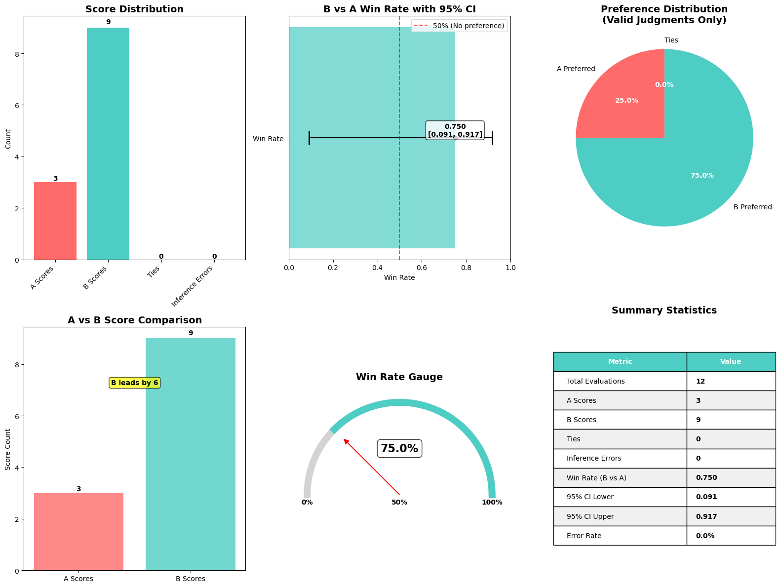
To assist practitioners rapidly interpret the result of a Nova LLM-as-a-Decide analysis, we created a comfort operate that produces a single, complete visualization summarizing key metrics. This operate, plot_nova_judge_results, makes use of Matplotlib and Seaborn to render a picture with six panels, every highlighting a special perspective of the analysis final result.

This operate takes the analysis metrics dictionary—produced when the analysis job is full—and generates the next visible parts:

  • Rating distribution bar chart – Reveals what number of occasions Mannequin A was most popular, what number of occasions Mannequin B was most popular, what number of ties occurred, and the way usually the decide failed to provide a choice (inference errors). This offers a right away sense of how decisive the analysis was and whether or not both mannequin is dominating.
  • Win fee with 95% confidence interval – Plots Mannequin B’s general win fee in opposition to Mannequin A, together with an error bar reflecting the decrease and higher bounds of the 95% confidence interval. A vertical reference line at 50% marks the purpose of no choice. If the boldness interval doesn’t cross this line, you’ll be able to conclude the result’s statistically important.
  • Choice pie chart – Visually shows the proportion of occasions Mannequin A, Mannequin B, or neither was most popular. This helps rapidly perceive choice distribution among the many legitimate judgments.
  • A vs. B rating comparability bar chart – Compares the uncooked counts of preferences for every mannequin facet by facet. A transparent label annotates the margin of distinction to emphasise which mannequin had extra wins.
  • Win fee gauge – Depicts the win fee as a semicircular gauge with a needle pointing to Mannequin B’s efficiency relative to the theoretical 0–100% vary. This intuitive visualization helps nontechnical stakeholders perceive the win fee at a look.
  • Abstract statistics desk – Compiles numerical metrics—together with complete evaluations, error counts, win fee, and confidence intervals—right into a compact, clear desk. This makes it simple to reference the precise numeric values behind the plots.

As a result of the operate outputs an ordinary Matplotlib determine, you’ll be able to rapidly save the picture, show it in Jupyter notebooks, or embed it in different documentation.

Clear up

Full the next steps to scrub up your sources:

  1. Delete your Qwen 2.5 1.5B Endpoint
    import boto3
    
    # Create a low-level SageMaker service consumer.
    
    sagemaker_client = boto3.consumer('sagemaker', region_name=)
    
    # Delete endpoint
    
    sagemaker_client.delete_endpoint(EndpointName=endpoint_name)

  2. In case you’re utilizing a SageMaker Studio JupyterLab pocket book, shut down the JupyterLab pocket book occasion.

How you should use this analysis framework

The Amazon Nova LLM-as-a-Decide workflow provides a dependable, repeatable manner to check two language fashions by yourself information. You may combine this into mannequin choice pipelines to determine which model performs greatest, or you’ll be able to schedule it as a part of steady analysis to catch regressions over time.

For groups constructing agentic or domain-specific programs, this method offers richer perception than automated metrics alone. As a result of your entire course of runs on SageMaker coaching jobs, it scales rapidly and produces clear visible studies that may be shared with stakeholders.

Conclusion

This put up demonstrates how Nova LLM-as-a-Decide—a specialised analysis mannequin out there via Amazon SageMaker AI—can be utilized to systematically measure the relative efficiency of generative AI programs. The walkthrough exhibits the right way to put together analysis datasets, launch SageMaker AI coaching jobs with Nova LLM-as-a-Decide recipes, and interpret the ensuing metrics, together with win charges and choice distributions. The totally managed SageMaker AI resolution simplifies this course of, so you’ll be able to run scalable, repeatable mannequin evaluations that align with human preferences.

We advocate beginning your LLM analysis journey by exploring the official Amazon Nova documentation and examples. The AWS AI/ML neighborhood provides intensive sources, together with workshops and technical steerage, to help your implementation journey.

To be taught extra, go to:


In regards to the authors

Surya Kari is a Senior Generative AI Knowledge Scientist at AWS, specializing in growing options leveraging state-of-the-art basis fashions. He has intensive expertise working with superior language fashions together with DeepSeek-R1, the Llama household, and Qwen, specializing in their fine-tuning and optimization. His experience extends to implementing environment friendly coaching pipelines and deployment methods utilizing AWS SageMaker. He collaborates with clients to design and implement generative AI options, serving to them navigate mannequin choice, fine-tuning approaches, and deployment methods to attain optimum efficiency for his or her particular use instances.

Joel Carlson is a Senior Utilized Scientist on the Amazon AGI basis modeling crew. He primarily works on growing novel approaches for enhancing the LLM-as-a-Decide functionality of the Nova household of fashions.

Saurabh Sahu is an utilized scientist within the Amazon AGI Basis modeling crew. He obtained his PhD in Electrical Engineering from College of Maryland Faculty Park in 2019. He has a background in multi-modal machine studying engaged on speech recognition, sentiment evaluation and audio/video understanding. Presently, his work focuses on growing recipes to enhance the efficiency of LLM-as-a-judge fashions for varied duties.

Morteza Ziyadi is an Utilized Science Supervisor at Amazon AGI, the place he leads a number of initiatives on post-training recipes and (Multimodal) massive language fashions within the Amazon AGI Basis modeling crew. Earlier than becoming a member of Amazon AGI, he spent 4 years at Microsoft Cloud and AI, the place he led initiatives targeted on growing pure language-to-code technology fashions for varied merchandise. He has additionally served as an adjunct school at Northeastern College. He earned his PhD from the College of Southern California (USC) in 2017 and has since been actively concerned as a workshop organizer, and reviewer for quite a few NLP, Laptop Imaginative and prescient and machine studying conferences.

Pradeep Natarajan is a Senior Principal Scientist in Amazon AGI Basis modeling crew engaged on post-training recipes and Multimodal massive language fashions. He has 20+ years of expertise in growing and launching a number of large-scale machine studying programs. He has a PhD in Laptop Science from College of Southern California.

Michael Cai is a Software program Engineer on the Amazon AGI Customization Group supporting the event of analysis options. He obtained his MS in Laptop Science from New York College in 2024. In his spare time he enjoys 3d printing and exploring modern tech.

Time collection prediction with FNN-LSTM


Right this moment, we decide up on the plan alluded to within the conclusion of the current Deep attractors: The place deep studying meets
chaos
: make use of that very same method to generate forecasts for
empirical time collection information.

“That very same method,” which for conciseness, I’ll take the freedom of referring to as FNN-LSTM, is because of William Gilpin’s
2020 paper “Deep reconstruction of unusual attractors from time collection” (Gilpin 2020).

In a nutshell, the issue addressed is as follows: A system, identified or assumed to be nonlinear and extremely depending on
preliminary circumstances, is noticed, leading to a scalar collection of measurements. The measurements should not simply – inevitably –
noisy, however as well as, they’re – at greatest – a projection of a multidimensional state house onto a line.

Classically in nonlinear time collection evaluation, such scalar collection of observations are augmented by supplementing, at each
time limit, delayed measurements of that very same collection – a way referred to as delay coordinate embedding (Sauer, Yorke, and Casdagli 1991). For
instance, as a substitute of only a single vector X1, we may have a matrix of vectors X1, X2, and X3, with X2 containing
the identical values as X1, however ranging from the third remark, and X3, from the fifth. On this case, the delay can be
2, and the embedding dimension, 3. Varied theorems state that if these
parameters are chosen adequately, it’s doable to reconstruct the whole state house. There’s a downside although: The
theorems assume that the dimensionality of the true state house is understood, which in lots of real-world functions, received’t be the
case.

That is the place Gilpin’s thought is available in: Practice an autoencoder, whose intermediate illustration encapsulates the system’s
attractor. Not simply any MSE-optimized autoencoder although. The latent illustration is regularized by false nearest
neighbors
(FNN) loss, a way generally used with delay coordinate embedding to find out an enough embedding dimension.
False neighbors are those that are shut in n-dimensional house, however considerably farther aside in n+1-dimensional house.
Within the aforementioned introductory submit, we confirmed how this
method allowed to reconstruct the attractor of the (artificial) Lorenz system. Now, we wish to transfer on to prediction.

We first describe the setup, together with mannequin definitions, coaching procedures, and information preparation. Then, we let you know the way it
went.

Setup

From reconstruction to forecasting, and branching out into the actual world

Within the earlier submit, we skilled an LSTM autoencoder to generate a compressed code, representing the attractor of the system.
As regular with autoencoders, the goal when coaching is similar because the enter, which means that general loss consisted of two
parts: The FNN loss, computed on the latent illustration solely, and the mean-squared-error loss between enter and
output. Now for prediction, the goal consists of future values, as many as we want to predict. Put in a different way: The
structure stays the identical, however as a substitute of reconstruction we carry out prediction, in the usual RNN manner. The place the standard RNN
setup would simply instantly chain the specified variety of LSTMs, we have now an LSTM encoder that outputs a (timestep-less) latent
code, and an LSTM decoder that ranging from that code, repeated as many instances as required, forecasts the required variety of
future values.

This after all signifies that to guage forecast efficiency, we have to examine towards an LSTM-only setup. That is precisely
what we’ll do, and comparability will become attention-grabbing not simply quantitatively, however qualitatively as nicely.

We carry out these comparisons on the 4 datasets Gilpin selected to reveal attractor reconstruction on observational
information
. Whereas all of those, as is obvious from the pictures
in that pocket book, exhibit good attractors, we’ll see that not all of them are equally suited to forecasting utilizing easy
RNN-based architectures – with or with out FNN regularization. However even people who clearly demand a special method enable
for attention-grabbing observations as to the influence of FNN loss.

Mannequin definitions and coaching setup

In all 4 experiments, we use the identical mannequin definitions and coaching procedures, the one differing parameter being the
variety of timesteps used within the LSTMs (for causes that can turn into evident after we introduce the person datasets).

Each architectures have been chosen to be simple, and about comparable in variety of parameters – each principally consist
of two LSTMs with 32 items (n_recurrent shall be set to 32 for all experiments).

FNN-LSTM

FNN-LSTM appears to be like practically like within the earlier submit, other than the truth that we break up up the encoder LSTM into two, to uncouple
capability (n_recurrent) from maximal latent state dimensionality (n_latent, saved at 10 identical to earlier than).

# DL-related packages
library(tensorflow)
library(keras)
library(tfdatasets)
library(tfautograph)
library(reticulate)

# going to wish these later
library(tidyverse)
library(cowplot)

encoder_model <- perform(n_timesteps,
                          n_features,
                          n_recurrent,
                          n_latent,
                          title = NULL) {
  
  keras_model_custom(title = title, perform(self) {
    
    self$noise <- layer_gaussian_noise(stddev = 0.5)
    self$lstm1 <-  layer_lstm(
      items = n_recurrent,
      input_shape = c(n_timesteps, n_features),
      return_sequences = TRUE
    ) 
    self$batchnorm1 <- layer_batch_normalization()
    self$lstm2 <-  layer_lstm(
      items = n_latent,
      return_sequences = FALSE
    ) 
    self$batchnorm2 <- layer_batch_normalization()
    
    perform (x, masks = NULL) {
      x %>%
        self$noise() %>%
        self$lstm1() %>%
        self$batchnorm1() %>%
        self$lstm2() %>%
        self$batchnorm2() 
    }
  })
}

decoder_model <- perform(n_timesteps,
                          n_features,
                          n_recurrent,
                          n_latent,
                          title = NULL) {
  
  keras_model_custom(title = title, perform(self) {
    
    self$repeat_vector <- layer_repeat_vector(n = n_timesteps)
    self$noise <- layer_gaussian_noise(stddev = 0.5)
    self$lstm <- layer_lstm(
      items = n_recurrent,
      return_sequences = TRUE,
      go_backwards = TRUE
    ) 
    self$batchnorm <- layer_batch_normalization()
    self$elu <- layer_activation_elu() 
    self$time_distributed <- time_distributed(layer = layer_dense(items = n_features))
    
    perform (x, masks = NULL) {
      x %>%
        self$repeat_vector() %>%
        self$noise() %>%
        self$lstm() %>%
        self$batchnorm() %>%
        self$elu() %>%
        self$time_distributed()
    }
  })
}

n_latent <- 10L
n_features <- 1
n_hidden <- 32

encoder <- encoder_model(n_timesteps,
                         n_features,
                         n_hidden,
                         n_latent)

decoder <- decoder_model(n_timesteps,
                         n_features,
                         n_hidden,
                         n_latent)

The regularizer, FNN loss, is unchanged:

loss_false_nn <- perform(x) {
  
  # altering these parameters is equal to
  # altering the power of the regularizer, so we maintain these fastened (these values
  # correspond to the unique values utilized in Kennel et al 1992).
  rtol <- 10 
  atol <- 2
  k_frac <- 0.01
  
  okay <- max(1, ground(k_frac * batch_size))
  
  ## Vectorized model of distance matrix calculation
  tri_mask <-
    tf$linalg$band_part(
      tf$ones(
        form = c(tf$forged(n_latent, tf$int32), tf$forged(n_latent, tf$int32)),
        dtype = tf$float32
      ),
      num_lower = -1L,
      num_upper = 0L
    )
  
  # latent x batch_size x latent
  batch_masked <-
    tf$multiply(tri_mask[, tf$newaxis,], x[tf$newaxis, reticulate::py_ellipsis()])
  
  # latent x batch_size x 1
  x_squared <-
    tf$reduce_sum(batch_masked * batch_masked,
                  axis = 2L,
                  keepdims = TRUE)
  
  # latent x batch_size x batch_size
  pdist_vector <- x_squared + tf$transpose(x_squared, perm = c(0L, 2L, 1L)) -
    2 * tf$matmul(batch_masked, tf$transpose(batch_masked, perm = c(0L, 2L, 1L)))
  
  #(latent, batch_size, batch_size)
  all_dists <- pdist_vector
  # latent
  all_ra <-
    tf$sqrt((1 / (
      batch_size * tf$vary(1, 1 + n_latent, dtype = tf$float32)
    )) *
      tf$reduce_sum(tf$sq.(
        batch_masked - tf$reduce_mean(batch_masked, axis = 1L, keepdims = TRUE)
      ), axis = c(1L, 2L)))
  
  # Keep away from singularity within the case of zeros
  #(latent, batch_size, batch_size)
  all_dists <-
    tf$clip_by_value(all_dists, 1e-14, tf$reduce_max(all_dists))
  
  #inds = tf.argsort(all_dists, axis=-1)
  top_k <- tf$math$top_k(-all_dists, tf$forged(okay + 1, tf$int32))
  # (#(latent, batch_size, batch_size)
  top_indices <- top_k[[1]]
  
  #(latent, batch_size, batch_size)
  neighbor_dists_d <-
    tf$collect(all_dists, top_indices, batch_dims = -1L)
  #(latent - 1, batch_size, batch_size)
  neighbor_new_dists <-
    tf$collect(all_dists[2:-1, , ],
              top_indices[1:-2, , ],
              batch_dims = -1L)
  
  # Eq. 4 of Kennel et al.
  #(latent - 1, batch_size, batch_size)
  scaled_dist <- tf$sqrt((
    tf$sq.(neighbor_new_dists) -
      # (9, 8, 2)
      tf$sq.(neighbor_dists_d[1:-2, , ])) /
      # (9, 8, 2)
      tf$sq.(neighbor_dists_d[1:-2, , ])
  )
  
  # Kennel situation #1
  #(latent - 1, batch_size, batch_size)
  is_false_change <- (scaled_dist > rtol)
  # Kennel situation 2
  #(latent - 1, batch_size, batch_size)
  is_large_jump <-
    (neighbor_new_dists > atol * all_ra[1:-2, tf$newaxis, tf$newaxis])
  
  is_false_neighbor <-
    tf$math$logical_or(is_false_change, is_large_jump)
  #(latent - 1, batch_size, 1)
  total_false_neighbors <-
    tf$forged(is_false_neighbor, tf$int32)[reticulate::py_ellipsis(), 2:(k + 2)]
  
  # Pad zero to match dimensionality of latent house
  # (latent - 1)
  reg_weights <-
    1 - tf$reduce_mean(tf$forged(total_false_neighbors, tf$float32), axis = c(1L, 2L))
  # (latent,)
  reg_weights <- tf$pad(reg_weights, record(record(1L, 0L)))
  
  # Discover batch common exercise
  
  # L2 Exercise regularization
  activations_batch_averaged <-
    tf$sqrt(tf$reduce_mean(tf$sq.(x), axis = 0L))
  
  loss <- tf$reduce_sum(tf$multiply(reg_weights, activations_batch_averaged))
  loss
  
}

Coaching is unchanged as nicely, other than the truth that now, we regularly output latent variable variances along with
the losses. It’s because with FNN-LSTM, we have now to decide on an enough weight for the FNN loss element. An “enough
weight” is one the place the variance drops sharply after the primary n variables, with n thought to correspond to attractor
dimensionality. For the Lorenz system mentioned within the earlier submit, that is how these variances regarded:

     V1       V2        V3        V4        V5        V6        V7        V8        V9       V10
 0.0739   0.0582   1.12e-6   3.13e-4   1.43e-5   1.52e-8   1.35e-6   1.86e-4   1.67e-4   4.39e-5

If we take variance as an indicator of significance, the primary two variables are clearly extra essential than the remainder. This
discovering properly corresponds to “official” estimates of Lorenz attractor dimensionality. For instance, the correlation dimension
is estimated to lie round 2.05 (Grassberger and Procaccia 1983).

Thus, right here we have now the coaching routine:

train_step <- perform(batch) {
  with (tf$GradientTape(persistent = TRUE) %as% tape, {
    code <- encoder(batch[[1]])
    prediction <- decoder(code)
    
    l_mse <- mse_loss(batch[[2]], prediction)
    l_fnn <- loss_false_nn(code)
    loss <- l_mse + fnn_weight * l_fnn
  })
  
  encoder_gradients <-
    tape$gradient(loss, encoder$trainable_variables)
  decoder_gradients <-
    tape$gradient(loss, decoder$trainable_variables)
  
  optimizer$apply_gradients(purrr::transpose(record(
    encoder_gradients, encoder$trainable_variables
  )))
  optimizer$apply_gradients(purrr::transpose(record(
    decoder_gradients, decoder$trainable_variables
  )))
  
  train_loss(loss)
  train_mse(l_mse)
  train_fnn(l_fnn)
  
  
}

training_loop <- tf_function(autograph(perform(ds_train) {
  for (batch in ds_train) {
    train_step(batch)
  }
  
  tf$print("Loss: ", train_loss$end result())
  tf$print("MSE: ", train_mse$end result())
  tf$print("FNN loss: ", train_fnn$end result())
  
  train_loss$reset_states()
  train_mse$reset_states()
  train_fnn$reset_states()
  
}))


mse_loss <-
  tf$keras$losses$MeanSquaredError(discount = tf$keras$losses$Discount$SUM)

train_loss <- tf$keras$metrics$Imply(title = 'train_loss')
train_fnn <- tf$keras$metrics$Imply(title = 'train_fnn')
train_mse <-  tf$keras$metrics$Imply(title = 'train_mse')

# fnn_multiplier needs to be chosen individually per dataset
# that is the worth we used on the geyser dataset
fnn_multiplier <- 0.7
fnn_weight <- fnn_multiplier * nrow(x_train)/batch_size

# studying charge may additionally want adjustment
optimizer <- optimizer_adam(lr = 1e-3)

for (epoch in 1:200) {
 cat("Epoch: ", epoch, " -----------n")
 training_loop(ds_train)
 
 test_batch <- as_iterator(ds_test) %>% iter_next()
 encoded <- encoder(test_batch[[1]]) 
 test_var <- tf$math$reduce_variance(encoded, axis = 0L)
 print(test_var %>% as.numeric() %>% spherical(5))
}

On to what we’ll use as a baseline for comparability.

Vanilla LSTM

Right here is the vanilla LSTM, stacking two layers, every, once more, of measurement 32. Dropout and recurrent dropout have been chosen individually
per dataset, as was the training charge.

lstm <- perform(n_latent, n_timesteps, n_features, n_recurrent, dropout, recurrent_dropout,
                 optimizer = optimizer_adam(lr =  1e-3)) {
  
  mannequin <- keras_model_sequential() %>%
    layer_lstm(
      items = n_recurrent,
      input_shape = c(n_timesteps, n_features),
      dropout = dropout, 
      recurrent_dropout = recurrent_dropout,
      return_sequences = TRUE
    ) %>% 
    layer_lstm(
      items = n_recurrent,
      dropout = dropout,
      recurrent_dropout = recurrent_dropout,
      return_sequences = TRUE
    ) %>% 
    time_distributed(layer_dense(items = 1))
  
  mannequin %>%
    compile(
      loss = "mse",
      optimizer = optimizer
    )
  mannequin
  
}

mannequin <- lstm(n_latent, n_timesteps, n_features, n_hidden, dropout = 0.2, recurrent_dropout = 0.2)

Information preparation

For all experiments, information have been ready in the identical manner.

In each case, we used the primary 10000 measurements obtainable within the respective .pkl information offered by Gilpin in his GitHub
repository
. To save lots of on file measurement and never rely upon an exterior
information supply, we extracted these first 10000 entries to .csv information downloadable instantly from this weblog’s repo:

geyser <- obtain.file(
  "https://uncooked.githubusercontent.com/rstudio/ai-blog/grasp/docs/posts/2020-07-20-fnn-lstm/information/geyser.csv",
  "information/geyser.csv")

electrical energy <- obtain.file(
  "https://uncooked.githubusercontent.com/rstudio/ai-blog/grasp/docs/posts/2020-07-20-fnn-lstm/information/electrical energy.csv",
  "information/electrical energy.csv")

ecg <- obtain.file(
  "https://uncooked.githubusercontent.com/rstudio/ai-blog/grasp/docs/posts/2020-07-20-fnn-lstm/information/ecg.csv",
  "information/ecg.csv")

mouse <- obtain.file(
  "https://uncooked.githubusercontent.com/rstudio/ai-blog/grasp/docs/posts/2020-07-20-fnn-lstm/information/mouse.csv",
  "information/mouse.csv")

Must you wish to entry the whole time collection (of significantly larger lengths), simply obtain them from Gilpin’s repo
and cargo them utilizing reticulate:

Right here is the info preparation code for the primary dataset, geyser – all different datasets have been handled the identical manner.

# the primary 10000 measurements from the compilation offered by Gilpin
geyser <- read_csv("geyser.csv", col_names = FALSE) %>% choose(X1) %>% pull() %>% unclass()

# standardize
geyser <- scale(geyser)

# varies per dataset; see beneath 
n_timesteps <- 60
batch_size <- 32

# remodel into [batch_size, timesteps, features] format required by RNNs
gen_timesteps <- perform(x, n_timesteps) {
  do.name(rbind,
          purrr::map(seq_along(x),
                     perform(i) {
                       begin <- i
                       finish <- i + n_timesteps - 1
                       out <- x[start:end]
                       out
                     })
  ) %>%
    na.omit()
}

n <- 10000
practice <- gen_timesteps(geyser[1:(n/2)], 2 * n_timesteps)
take a look at <- gen_timesteps(geyser[(n/2):n], 2 * n_timesteps) 

dim(practice) <- c(dim(practice), 1)
dim(take a look at) <- c(dim(take a look at), 1)

# break up into enter and goal  
x_train <- practice[ , 1:n_timesteps, , drop = FALSE]
y_train <- practice[ , (n_timesteps + 1):(2*n_timesteps), , drop = FALSE]

x_test <- take a look at[ , 1:n_timesteps, , drop = FALSE]
y_test <- take a look at[ , (n_timesteps + 1):(2*n_timesteps), , drop = FALSE]

# create tfdatasets
ds_train <- tensor_slices_dataset(record(x_train, y_train)) %>%
  dataset_shuffle(nrow(x_train)) %>%
  dataset_batch(batch_size)

ds_test <- tensor_slices_dataset(record(x_test, y_test)) %>%
  dataset_batch(nrow(x_test))

Now we’re prepared to have a look at how forecasting goes on our 4 datasets.

Experiments

Geyser dataset

Folks working with time collection could have heard of Outdated Trustworthy, a geyser in
Wyoming, US that has regularly been erupting each 44 minutes to 2 hours because the yr 2004. For the subset of information
Gilpin extracted,

geyser_train_test.pkl corresponds to detrended temperature readings from the principle runoff pool of the Outdated Trustworthy geyser
in Yellowstone Nationwide Park, downloaded from the GeyserTimes database. Temperature measurements
begin on April 13, 2015 and happen in one-minute increments.

Like we mentioned above, geyser.csv is a subset of those measurements, comprising the primary 10000 information factors. To decide on an
enough timestep for the LSTMs, we examine the collection at varied resolutions:

Determine 1: Geyer dataset. High: First 1000 observations. Backside: Zooming in on the primary 200.

It looks as if the habits is periodic with a interval of about 40-50; a timestep of 60 thus appeared like a very good strive.

Having skilled each FNN-LSTM and the vanilla LSTM for 200 epochs, we first examine the variances of the latent variables on
the take a look at set. The worth of fnn_multiplier akin to this run was 0.7.

test_batch <- as_iterator(ds_test) %>% iter_next()
encoded <- encoder(test_batch[[1]]) %>%
  as.array() %>%
  as_tibble()

encoded %>% summarise_all(var)
   V1     V2        V3          V4       V5       V6       V7       V8       V9      V10
0.258 0.0262 0.0000627 0.000000600 0.000533 0.000362 0.000238 0.000121 0.000518 0.000365

There’s a drop in significance between the primary two variables and the remainder; nonetheless, not like within the Lorenz system, V1 and
V2 variances additionally differ by an order of magnitude.

Now, it’s attention-grabbing to match prediction errors for each fashions. We’re going to make a remark that can carry
by means of to all three datasets to return.

Maintaining the suspense for some time, right here is the code used to compute per-timestep prediction errors from each fashions. The
similar code shall be used for all different datasets.

calc_mse <- perform(df, y_true, y_pred) {
  (sum((df[[y_true]] - df[[y_pred]])^2))/nrow(df)
}

get_mse <- perform(test_batch, prediction) {
  
  comp_df <- 
    information.body(
      test_batch[[2]][, , 1] %>%
        as.array()) %>%
        rename_with(perform(title) paste0(title, "_true")) %>%
    bind_cols(
      information.body(
        prediction[, , 1] %>%
          as.array()) %>%
          rename_with(perform(title) paste0(title, "_pred")))
  
  mse <- purrr::map(1:dim(prediction)[2],
                        perform(varno)
                          calc_mse(comp_df,
                                   paste0("X", varno, "_true"),
                                   paste0("X", varno, "_pred"))) %>%
    unlist()
  
  mse
}

prediction_fnn <- decoder(encoder(test_batch[[1]]))
mse_fnn <- get_mse(test_batch, prediction_fnn)

prediction_lstm <- mannequin %>% predict(ds_test)
mse_lstm <- get_mse(test_batch, prediction_lstm)

mses <- information.body(timestep = 1:n_timesteps, fnn = mse_fnn, lstm = mse_lstm) %>%
  collect(key = "sort", worth = "mse", -timestep)

ggplot(mses, aes(timestep, mse, coloration = sort)) +
  geom_point() +
  scale_color_manual(values = c("#00008B", "#3CB371")) +
  theme_classic() +
  theme(legend.place = "none") 

And right here is the precise comparability. One factor particularly jumps to the attention: FNN-LSTM forecast error is considerably decrease for
preliminary timesteps, at the start, for the very first prediction, which from this graph we anticipate to be fairly good!


Per-timestep prediction error as obtained by FNN-LSTM and a vanilla stacked LSTM. Green: LSTM. Blue: FNN-LSTM.

Determine 2: Per-timestep prediction error as obtained by FNN-LSTM and a vanilla stacked LSTM. Inexperienced: LSTM. Blue: FNN-LSTM.

Curiously, we see “jumps” in prediction error, for FNN-LSTM, between the very first forecast and the second, after which
between the second and the following ones, reminding of the same jumps in variable significance for the latent code! After the
first ten timesteps, vanilla LSTM has caught up with FNN-LSTM, and we received’t interpret additional improvement of the losses primarily based
on only a single run’s output.

As an alternative, let’s examine precise predictions. We randomly decide sequences from the take a look at set, and ask each FNN-LSTM and vanilla
LSTM for a forecast. The identical process shall be adopted for the opposite datasets.

given <- information.body(as.array(tf$concat(record(
  test_batch[[1]][, , 1], test_batch[[2]][, , 1]
),
axis = 1L)) %>% t()) %>%
  add_column(sort = "given") %>%
  add_column(num = 1:(2 * n_timesteps))

fnn <- information.body(as.array(prediction_fnn[, , 1]) %>%
                    t()) %>%
  add_column(sort = "fnn") %>%
  add_column(num = (n_timesteps  + 1):(2 * n_timesteps))

lstm <- information.body(as.array(prediction_lstm[, , 1]) %>%
                     t()) %>%
  add_column(sort = "lstm") %>%
  add_column(num = (n_timesteps + 1):(2 * n_timesteps))

compare_preds_df <- bind_rows(given, lstm, fnn)

plots <- 
  purrr::map(pattern(1:dim(compare_preds_df)[2], 16),
             perform(v) {
               ggplot(compare_preds_df, aes(num, .information[[paste0("X", v)]], coloration = sort)) +
                 geom_line() +
                 theme_classic() +
                 theme(legend.place = "none", axis.title = element_blank()) +
                 scale_color_manual(values = c("#00008B", "#DB7093", "#3CB371"))
             })

plot_grid(plotlist = plots, ncol = 4)

Listed here are sixteen random picks of predictions on the take a look at set. The bottom reality is displayed in pink; blue forecasts are from
FNN-LSTM, inexperienced ones from vanilla LSTM.


60-step ahead predictions from FNN-LSTM (blue) and vanilla LSTM (green) on randomly selected sequences from the test set. Pink: the ground truth.

Determine 3: 60-step forward predictions from FNN-LSTM (blue) and vanilla LSTM (inexperienced) on randomly chosen sequences from the take a look at set. Pink: the bottom reality.

What we anticipate from the error inspection comes true: FNN-LSTM yields considerably higher predictions for rapid
continuations of a given sequence.

Let’s transfer on to the second dataset on our record.

Electrical energy dataset

This can be a dataset on energy consumption, aggregated over 321 totally different households and fifteen-minute-intervals.

electricity_train_test.pkl corresponds to common energy consumption by 321 Portuguese households between 2012 and 2014, in
items of kilowatts consumed in fifteen minute increments. This dataset is from the UCI machine studying
database
.

Right here, we see a really common sample:


Electricity dataset. Top: First 2000 observations. Bottom: Zooming in on 500 observations, skipping the very beginning of the series.

Determine 4: Electrical energy dataset. High: First 2000 observations. Backside: Zooming in on 500 observations, skipping the very starting of the collection.

With such common habits, we instantly tried to foretell the next variety of timesteps (120) – and didn’t should retract
behind that aspiration.

For an fnn_multiplier of 0.5, latent variable variances appear like this:

V1          V2            V3       V4       V5            V6       V7         V8      V9     V10
0.390 0.000637 0.00000000288 1.48e-10 2.10e-11 0.00000000119 6.61e-11 0.00000115 1.11e-4 1.40e-4

We undoubtedly see a pointy drop already after the primary variable.

How do prediction errors examine on the 2 architectures?


Per-timestep prediction error as obtained by FNN-LSTM and a vanilla stacked LSTM. Green: LSTM. Blue: FNN-LSTM.

Determine 5: Per-timestep prediction error as obtained by FNN-LSTM and a vanilla stacked LSTM. Inexperienced: LSTM. Blue: FNN-LSTM.

Right here, FNN-LSTM performs higher over an extended vary of timesteps, however once more, the distinction is most seen for rapid
predictions. Will an inspection of precise predictions affirm this view?


60-step ahead predictions from FNN-LSTM (blue) and vanilla LSTM (green) on randomly selected sequences from the test set. Pink: the ground truth.

Determine 6: 60-step forward predictions from FNN-LSTM (blue) and vanilla LSTM (inexperienced) on randomly chosen sequences from the take a look at set. Pink: the bottom reality.

It does! In truth, forecasts from FNN-LSTM are very spectacular on all time scales.

Now that we’ve seen the straightforward and predictable, let’s method the bizarre and troublesome.

ECG dataset

Says Gilpin,

ecg_train.pkl and ecg_test.pkl correspond to ECG measurements for 2 totally different sufferers, taken from the PhysioNet QT
database
.

How do these look?


ECG dataset. Top: First 1000 observations. Bottom: Zooming in on the first 400 observations.

Determine 7: ECG dataset. High: First 1000 observations. Backside: Zooming in on the primary 400 observations.

To the layperson that I’m, these don’t look practically as common as anticipated. First experiments confirmed that each architectures
should not able to coping with a excessive variety of timesteps. In each strive, FNN-LSTM carried out higher for the very first
timestep.

That is additionally the case for n_timesteps = 12, the ultimate strive (after 120, 60 and 30). With an fnn_multiplier of 1, the
latent variances obtained amounted to the next:

     V1        V2          V3        V4         V5       V6       V7         V8         V9       V10
  0.110  1.16e-11     3.78e-9 0.0000992    9.63e-9  4.65e-5  1.21e-4    9.91e-9    3.81e-9   2.71e-8

There is a niche between the primary variable and all different ones; however not a lot variance is defined by V1 both.

Aside from the very first prediction, vanilla LSTM exhibits decrease forecast errors this time; nonetheless, we have now so as to add that this
was not constantly noticed when experimenting with different timestep settings.


Per-timestep prediction error as obtained by FNN-LSTM and a vanilla stacked LSTM. Green: LSTM. Blue: FNN-LSTM.

Determine 8: Per-timestep prediction error as obtained by FNN-LSTM and a vanilla stacked LSTM. Inexperienced: LSTM. Blue: FNN-LSTM.

precise predictions, each architectures carry out greatest when a persistence forecast is enough – in truth, they
produce one even when it’s not.


60-step ahead predictions from FNN-LSTM (blue) and vanilla LSTM (green) on randomly selected sequences from the test set. Pink: the ground truth.

Determine 9: 60-step forward predictions from FNN-LSTM (blue) and vanilla LSTM (inexperienced) on randomly chosen sequences from the take a look at set. Pink: the bottom reality.

On this dataset, we definitely would wish to discover different architectures higher capable of seize the presence of excessive and low
frequencies within the information, corresponding to combination fashions. However – have been we compelled to stick with considered one of these, and will do a
one-step-ahead, rolling forecast, we’d go along with FNN-LSTM.

Talking of blended frequencies – we haven’t seen the extremes but …

Mouse dataset

“Mouse,” that’s spike charges recorded from a mouse thalamus.

mouse.pkl A time collection of spiking charges for a neuron in a mouse thalamus. Uncooked spike information was obtained from
CRCNS and processed with the authors’ code with a view to generate a
spike charge time collection.


Mouse dataset. Top: First 2000 observations. Bottom: Zooming in on the first 500 observations.

Determine 10: Mouse dataset. High: First 2000 observations. Backside: Zooming in on the primary 500 observations.

Clearly, this dataset shall be very laborious to foretell. How, after “lengthy” silence, are you aware {that a} neuron goes to fireside?

As regular, we examine latent code variances (fnn_multiplier was set to 0.4):

Whereas it’s straightforward to acquire these estimates, utilizing, for example, the
nonlinearTseries bundle explicitly modeled after practices
described in Kantz & Schreiber’s basic (Kantz and Schreiber 2004), we don’t wish to extrapolate from our tiny pattern of datasets, and go away
such explorations and analyses to additional posts, and/or the reader’s ventures :-). In any case, we hope you loved
the demonstration of sensible usability of an method that within the previous submit, was primarily launched when it comes to its
conceptual attractivity.

Thanks for studying!

Gilpin, William. 2020. “Deep Reconstruction of Unusual Attractors from Time Sequence.” https://arxiv.org/abs/2002.05909.
Grassberger, Peter, and Itamar Procaccia. 1983. “Measuring the Strangeness of Unusual Attractors.” Physica D: Nonlinear Phenomena 9 (1): 189–208. https://doi.org/https://doi.org/10.1016/0167-2789(83)90298-1.

Kantz, Holger, and Thomas Schreiber. 2004. Nonlinear Time Sequence Evaluation. Cambridge College Press.

Sauer, Tim, James A. Yorke, and Martin Casdagli. 1991. Embedology.” Journal of Statistical Physics 65 (3-4): 579–616. https://doi.org/10.1007/BF01053745.