I blogged about this information beforehand, and I’m returning to it now as a part of my semi-regular Dialogue Board Concepts collection on this weblog. I’ve been utilizing this immediate in my on-line stats class in NW PA for a couple of yr now. I will share a few of that success right here. Observe: PA is #4 for deer-related automobile accident claims, so this information resonates with my college students.
I take advantage of this for the fifth of seven weeks in my on-line class, so the scholars are comfy with the category format and each other by then. Right here is the precise immediate I take advantage of:
I’ve a bizarre query for you: How do you suppose Pennsylvania ranks in the case of the variety of automobile accident insurance coverage claims involving colliding with animals? Sure, I’m on my soapbox about protected night-time driving in PA.
After you have your guess, examine towards the actual reply right here: https://www.statefarm.com/simple-insights/auto-and-vehicles/how-likely-are-you-to-have-an-animal-collision
For the larger dialogue, how do you suppose this information ought to inform insurance coverage charges? Public security/driving funding? How ought to it inform your driving?
College students can actually dig into this. Listed here are a couple of of the issues I get pleasure from essentially the most about utilizing this information:
1) Worldwide college students/out of state college students/metropolis slickers GET THIS DATA. Like, if you happen to do not develop up seeing lots of deer roadkill each day, it’s fairly appalling to come across the primary couple of occasions. It makes an impression, and college students share these tales within the dialogue board. I bear in mind one in every of my out-of-state college students on the soccer group commenting on the variety of lifeless deer he noticed out the group bus window whereas touring to rural PA faculties and universities for video games.
2) Native college students get this information, too. Within the dialogue board, college students recount their very own automobile accidents and close to misses, which will get the scholars speaking within the dialogue as an alternative of simply complimenting and agreeing with one another. Generally, fundamental engagement is difficult to return by with dialogue boards in a stats class. This is the reason I’ve switched to dialogue boards that use only one vivid instance to explain how information may be useful in actual life. I used to have extra in-depth dialogue boards, however I believe briefer dialogue boards higher convey the urgency and fascination I really feel when pondering information.
3) College students go from not even figuring out this information exists to brainstorming about prevention measures primarily based on this information. At any time when I take advantage of this dialogue board, I ask the scholars what to do with this information. My college students have many good concepts on how this information might inform apply: Maybe driver’s schooling lessons in deer-prone accident areas might train college students the right way to scan for deer whereas driving. There could possibly be PSAs throughout looking/breeding seasons so of us bear in mind to scan for deer. The PSAs might additionally remind drivers that if you happen to see one deer, there are in all probability different deer close by. College students have additionally advised that this information could possibly be used to information signage/lighting choices on rural highways the place there are frequent accidents. This information could possibly be used when setting budgets and prioritizing street enchancment tasks. This information is also used when distributing looking licenses and figuring out the variety of deer a hunter can bag per season.
4) When individuals in energy take into account how they’ll greatest use their authority to enhance everybody’s lives, they should bear in mind the wants of rural Individuals.
In the event you’re an utilized researcher, chances are high you’ve got used speculation testing earlier than. It is an important software in sensible functions — whether or not you are validating financial fashions, assessing coverage impacts, or making data-driven enterprise and monetary selections.
The ability of speculation testing lies in its means to offer a structured framework for making goal selections based mostly on knowledge quite than instinct or anecdotal proof. It permits us to systematically test the validity of our assumptions and fashions. The concept is easy — by formulating null and different hypotheses, we are able to decide whether or not noticed relationships between variables are statistically important or just on account of probability.
In in the present day’s weblog, we’ll take a better have a look at the statistical instinct behind speculation testing utilizing the Wald Take a look at and supply a step-by-step information for implementing speculation testing in GAUSS.
Understanding the Instinct of Speculation Testing
We don’t have to utterly perceive the mathematical background of speculation testing with the Wald Take a look at to make use of it successfully. Nevertheless, having some background will assist guarantee appropriate implementation and interpretation.
The Null Speculation
On the coronary heart of speculation testing is the null speculation. It formally represents the assumptions we need to check.
In mathematical phrases, it’s constructed as a set of linear restrictions on our parameters and is given by:
$$ H_0: Rbeta = q $$
the place:
$R$ is a matrix specifying the linear constraints on the parameters.
$q$ is a vector of hypothesized values.
$beta$ is the vector of mannequin parameters.
The null speculation captures two key items of data:
Data from our noticed knowledge, mirrored within the estimated mannequin parameters.
The assumptions we’re testing, represented by the linear constraints and hypothesized values.
The Wald Take a look at Statistic
After formulating the null speculation, the Wald Take a look at Statistic is computed as:
the place $hat{V}$ is the estimated variance-covariance matrix.
The Instinct of the Wald Take a look at Statistic
Let’s take a better have a look at the parts of the check statistic.
The primary element of the check statistic, $(Rhat{beta} – q)$, measures how a lot the noticed parameters differ from the null speculation:
If our constraints maintain precisely, $Rhat{beta} = q$, and the check statistic is zero.
As a result of the check statistic squares the deviation, it captures variations in both route.
The bigger this element, the farther the noticed knowledge are from the null speculation.
A bigger deviation results in a bigger check statistic.
The second element of the check statistic, $(Rhat{V}R’)^{-1}$, accounts for the variability in our knowledge:
Because the variability of our knowledge will increase, $(Rhat{V}R’)$ will increase.
For the reason that squared deviation is split by this element, a rise in variability results in a decrease check statistic. Intuitively, excessive variability implies that even a big deviation from the null speculation may not be statistically important.
Scaling by variability prevents us from rejecting the null speculation on account of excessive uncertainty within the estimates.
Notice that the GAUSS waldTest process makes use of the F-test different to the Wald Take a look at, which scales the Wald Statistic by the variety of restrictions.
Decoding the Wald Take a look at Statistic
Understanding the Wald Take a look at might help us higher interpret its outcomes. Usually, the bigger the Wald Take a look at statistic:
The additional our noticed knowledge deviates from $H_0$.
The much less possible our noticed knowledge are underneath $H_0$.
The extra possible we’re to reject $H_0$.
To make extra particular conclusions, we are able to use the p-value of our check statistic. The F-test different utilized by the GAUSS waldTest process follows an F distribution:
$$ F sim F(q, d) $$
the place:
$q$ is the variety of constraints.
$d$ is the residual levels of freedom.
The p-value, in comparison with a selected significance degree $alpha$, helps us decide whether or not to reject the null speculation. It represents the chance of observing a check statistic as excessive as (or extra excessive than) the calculated Wald Take a look at statistic, assuming the null speculation is true.
Thus:
If $p leq alpha$, we reject $H_0$.
If $p > alpha$, we fail to reject $H_0$.
The GAUSS waldTest Process
In GAUSS, speculation testing may be carried out utilizing the waldTest process, launched in GAUSS 25.
The waldTest process can be utilized in two methods:
Put up-estimation with a crammed output construction after estimation utilizing olsmt, gmmfit, glm, or quantilefit.
Straight, utilizing an estimated parameter vector and variance matrix.
Put up-estimation Utilization
If used post-estimation, the waldTest process has one required enter and 4 elective inputs:
Put up-estimation crammed output construction. Legitimate construction sorts embrace: olsmtOut, gmmOut, glmOut, and qfitOut.
R
Elective, LHS of the null speculation. Needs to be specified by way of the mannequin variables, with a separate row for every speculation. The perform accepts linear mixtures of the mannequin variables.
q
Elective, RHS of the null speculation. Have to be numeric vector.
tau
Elective, tau degree equivalent to the testing speculation. Default is to collectively checks throughout all tau values. Solely legitimate for the qfitOut construction.
joint
Elective, specification to check quantileFit hypotheses collectively throughout all coefficients for the qfitOut construction.
Information Matrices
If knowledge matrices are used, the waldTest process has two required inputs and 4 elective inputs:
Elective, LHS of the null speculation. Needs to be specified by way of the mannequin variables, with a separate row for every speculation. The perform accepts linear mixtures of the mannequin variables.
q
Elective, RHS of the null speculation. Have to be numeric vector.
df_residuals
Elective, mannequin levels of freedom for the F-test.
varnames
Elective, variable names.
Specifying The Null Speculation for Testing
By default, the waldTest process checks whether or not all estimated parameters collectively equal zero. This offers a fast technique to assess the general explanatory energy of a mannequin. Nevertheless, the true power of the waldTest process lies in its means to check any linear mixture of estimated parameters.
Specifying the speculation for testing is intuitive and may be performed utilizing variable names as a substitute of manually setting up constraint matrices. This user-friendly method:
Reduces errors.
Accelerates workflow.
Permits us to give attention to decoding outcomes quite than establishing complicated computations.
Now, let’s take a better have a look at the 2 inputs used to specify the null speculation: the R and q inputs.
The R Restriction Enter
The elective R enter specifies the restrictions to be examined. This enter:
Have to be a string array.
Ought to use your mannequin variable names.
Can embrace any linear mixture of the mannequin variables.
Ought to have one row for each speculation to be collectively examined.
and need to check whether or not the coefficients on weight and axles are equal.
To specify this restriction, we outline R as follows:
// Set R to check
// if the coefficient on weight
// and axles are equal (weight - axles = 0)
R = "weight - axles";
The q Enter
The elective q enter specifies the right-hand aspect (RHS) of the null speculation. By default, it checks whether or not all hypotheses have a worth of 0.
To check hypothesized values apart from zero, we should specify the q enter.
The q enter should:
Be a numerical vector.
Have one row for each speculation to be collectively examined.
Persevering with our earlier instance, suppose we need to check whether or not the coefficient on weight equals 2.
// Set R to check
// coefficient on weight = 2
R = "weight";

// Set hypothesized worth
// utilizing q
q = 2;
The waldTest Process in Motion
One of the simplest ways to familiarize ourselves with the waldTest process is thru hands-on examples. All through these examples, we’ll use a hypothetical dataset containing 4 variables: earnings, training, expertise, and hours.
Subsequent, we use waldtest to check our speculation:
// Take a look at if coefficients for training and expertise are equal
R = "training - expertise";
name waldTest(ols_out, R);
===================================
Wald check of null joint speculation:
training - expertise =  0
-----------------------------------
F( 1, 46 ):                  0.0978
Prob > F :                   0.7559
===================================
For the reason that check statistic is 0.0978 and the p-value is 0.756, we fail to reject the null speculation, suggesting that the coefficients are usually not considerably totally different.
Instance 2: Testing A number of Hypotheses After GLM
In our second instance, let’s use waldTest to check a number of hypotheses collectively after utilizing glm. We’ll estimate the identical mannequin as in our first instance. Nevertheless, this time we’ll use the waldTest process to collectively check two hypotheses:
Notice that these outcomes are equivalent to the primary instance as a result of we specified that GLM use the traditional household, which is equal to OLS.
Subsequent, we check our joint speculation. For this check, take into accout:
We should specify a q enter as a result of considered one of our hypothesized values is totally different from zero.
Our R and q inputs will every have two rows as a result of we’re collectively testing two hypotheses.
// Outline a number of hypotheses:
// 1. training - expertise = 0
// 2. training + expertise = 1
R = "training - expertise" $| "training + expertise";
q = 0 | 1;

// Carry out Wald check for joint hypotheses
name waldTest(glm_out, R, q);
===================================
Wald check of null joint speculation:

training - expertise =  0
training + hours      =  1
-----------------------------------
F( 2, 46 ):                  0.5001
Prob > F :                   0.6097
===================================
For the reason that check statistic is 0.5001 and the p-value is 0.6097:
We fail to reject the null speculation, indicating that the constraints maintain throughout the limits of statistical significance.
Our noticed knowledge doesn’t present statistical proof to conclude that both restriction is violated.
Instance 3: Utilizing Information Matrices
Whereas waldTest is handy to be used after GAUSS estimation procedures, there could also be circumstances the place we have to apply it after guide parameter computations. In such circumstances, we are able to enter our estimated parameters and covariance matrix immediately utilizing knowledge matrices.
// Run OLSMT estimation with guide computation of beta and sigma
X = ones(rows(knowledge), 1) ~ knowledge[., "education" "experience" "hours"];
y = knowledge[., "income"];

// Compute beta manually
params = invpd(X'X) * X'y;

// Compute residuals and sigma
residuals = y - X * params;
n = rows(y);
ok = cols(X);
sigma = (residuals'residuals) / (n - ok) * invpd(X'X);
We will now use the manually computed params and sigma with waldTest. Nevertheless, we should additionally present the next further info:
The residual levels of freedom.
The variable names.
// Outline speculation: training - expertise = 0
R = "training - expertise";
q = 0;

// Discover levels of freedom
df_residuals = n - ok;

// Specify variable names
varnames = "CONSTANT"$|"expertise"$|"training"$|"hours";

// Carry out Wald check
name waldTest(sigma, params, R, q, df_residuals, varnames);
===================================
Wald check of null joint speculation:
training - expertise =  0
-----------------------------------
F( 1, 46 ):                  0.0978
Prob > F :                   0.7559
===================================
As an alternative choice to specifying variable names, we might specify our speculation by way of default variable names, "X1, X2, ..., XK".
Conclusion
In in the present day’s weblog, we explored the instinct behind speculation testing and demonstrated how you can implement the Wald Take a look at in GAUSS utilizing the waldTest process.
We coated:
What the Wald Take a look at is and why it issues in statistical modeling.
Key options of the waldTest process.
Step-by-step examples of making use of waldTest after totally different estimation strategies.
The code and knowledge from this weblog may be discovered right here.
Eric( Director of Functions and Coaching at Aptech Programs, Inc. )
Eric has been working to construct, distribute, and strengthen the GAUSS universe since 2012. He’s an economist expert in knowledge evaluation and software program growth. He has earned a B.A. and MSc in economics and engineering and has over 18 years of mixed trade and tutorial expertise in knowledge evaluation and analysis.
Entry the code to this tutorial and all different 500+ tutorials on PyImageSearch
Enter your electronic mail deal with under to be taught extra about PyImageSearch College (together with how one can obtain the supply code to this publish):
What’s included in PyImageSearch College?
Quick access to the code, datasets, and pre-trained fashions for all 500+ tutorials on the PyImageSearch weblog
Excessive-quality, nicely documented supply code with line-by-line explanations (making certain precisely what the code is doing)
Jupyter Notebooks which are pre-configured to run in Google Colab with a single click on
Run all code examples in your net browser — no dev surroundings configuration required!
Assist for all main working techniques (Home windows, macOS, Linux, and Raspbian)
Full entry to PyImageSearch College programs
Detailed video tutorials for each lesson
Certificates of Completion for all programs
New programs added each month! — keep on high of state-of-the-art developments in pc imaginative and prescient and deep studying
PyImageSearch College is actually the most effective Laptop Visions “Masters” Diploma that I want I had when beginning out. Having the ability to entry all of Adrian’s tutorials in a single listed web page and having the ability to begin taking part in round with the code with out going by the nightmare of organising all the pieces is simply wonderful. 10/10 would suggest.
Sanyam BhutaniMachine Studying Engineer and 2x Kaggle Grasp
AWS responded shortly, rolling again modifications and isolating affected elements. Communications from AWS Assist, whereas well timed, have been predictably technical and lacked specifics because the disaster developed. Points with autoscaling, load balancing, and site visitors routing triggered downstream results on seemingly unrelated providers. It’s a reminder that, regardless of the concentrate on “resilience” and “availability zones,” cloud infrastructure remains to be topic to the identical basic legal guidelines of physics and software program vulnerabilities, similar to something in your individual information middle.
The ultimate decision got here just a few hours later, after community engineers manually rebalanced the distributed methods and verified the restoration of regular operations. Connectivity returned, however some prospects reported information inconsistencies, delayed API recoveries, and gradual catch-up occasions. The scramble to speak with shoppers, reset processes, and work by the backlog served as a harsh reminder: Enterprise continuity depends upon greater than hope and a strong advertising and marketing pitch out of your supplier.
The parable of the bulletproof SLA
Some companies hoped for quick cures from AWS’s legendary service-level agreements. Right here’s the truth: SLA credit are chilly consolation when your income pipeline is in freefall. The reality that each CIO has confronted not less than as soon as is that even industry-leading SLAs not often compensate for the true value of downtime. They don’t make up for misplaced alternatives, broken reputations, or the stress in your groups. As regional outages enhance as a result of progress of hyperscale cloud information facilities, every struggling to deal with the surge in AI-driven demand, the security web is changing into much less reliable.
That is at present’s version of The Obtain, our weekday e-newsletter that gives a day by day dose of what’s occurring on the earth of expertise.
What’s subsequent for carbon removing?
After years of progress that spawned a whole lot of startups, the nascent carbon removing sector seems to be dealing with a reckoning.
Operating Tide, a promising aquaculture firm, shut down its operations final summer season, and a handful of different firms have shuttered, downsized, or pivoted in current months as properly. Enterprise investments have flagged. And the collective trade hasn’t made a complete lot extra progress towards Operating Tide’s formidable plans to sequester a billion tons of carbon dioxide by this yr.
The hype section is over and the sector is sliding into the turbulent enterprise trough that follows, specialists warn.
And the open query is: If the carbon removing sector is heading right into a painful if inevitable clearing-out cycle, the place will it go from there? Learn the total story.
—James Temple
This story is a part of MIT Know-how Evaluation’s What’s Subsequent collection, which seems throughout industries, traits, and applied sciences to provide you a primary have a look at the long run. You’ll be able to learn the remainder of them right here.
An AI app to measure ache is right here
This week I’ve additionally been questioning how science and expertise can assist reply that query—particularly relating to ache.
Within the newest subject of MIT Know-how Evaluation’s print journal, Deena Mousa describes how an AI-powered smartphone app is getting used to evaluate how a lot ache an individual is in.
The app, and different instruments prefer it, might assist medical doctors and caregivers. They might be particularly helpful within the care of people that aren’t capable of inform others how they’re feeling.
However they’re removed from excellent. And so they open up all types of thorny questions on how we expertise, talk, and even deal with ache. Learn the total story.
—Jessica Hamzelou
This text first appeared in The Checkup, MIT Know-how Evaluation’s weekly biotech e-newsletter. To obtain it in your inbox each Thursday, and browse articles like this primary, enroll right here.
The must-reads
I’ve combed the web to search out you at present’s most enjoyable/vital/scary/fascinating tales about expertise.
1 Meta’s legal professionals suggested staff to take away elements of its teen psychological well being analysis Its counsel informed researchers to dam or replace their work to scale back authorized legal responsibility. (Bloomberg $) + Meta just lately laid off greater than 100 workers tasked with monitoring dangers to person privateness. (NYT $)
2 Donald Trump has pardoned the convicted Binance founder ChangpengZhao pleaded responsible to violating US cash laundering legal guidelines in 2023. (WSJ $) + The transfer is prone to allow Binance to renew working within the US. (CNN) + Trump has vowed to be extra crypto-friendly than the Biden administration. (Axios)
3 Anthropic and Google Cloud have signed a serious chips deal The settlement is price tens of billions of {dollars}. (FT $)
4 Microsoft doesn’t need you to speak soiled to its AI It’ll go away that sort of factor to OpenAI, thanks very a lot. (CNBC) + Copilot now has its personal model of Clippy—simply don’t attempt to get erotic with it. (The Verge) + It’s fairly simple to get DeepSeek to speak soiled, nevertheless. (MIT Know-how Evaluation)
5 Large Tech is footing the invoice for Trump’s White Home ballroom Arise Amazon, Apple, Google, Meta, and Microsoft. (TechCrunch) + Crypto twins Tyler and Cameron Winklevoss are additionally among the many donors. (CNN)
6 US investigators have busted a collection of high-tech playing schemes Involving specially-designed contact lenses and x-ray tables. (NYT $) + The case follows insider bets on basketball and poker video games rigged by the mafia. (BBC) + Automated card shufflers will be compromised, too. (Wired $)
7 Deepfake harassment instruments are simply accessible on social media And easy internet searches. (404 Media) + Bans on deepfakes take us solely to date—right here’s what we actually want. (MIT Know-how Evaluation)
8 How algorithms can drive up costs on-line Even benign algorithms can generally yield unhealthy outcomes for consumers. (Quanta Journal) + When AIs discount, a much less superior agent might value you. (MIT Know-how Evaluation)
9 How you can give an LLM mind rot Prepare it on quick “superficial” posts from X, for a begin. (Ars Technica) + AI skilled on AI rubbish spits out AI rubbish. (MIT Know-how Evaluation)
10 Meet the tech staff utilizing AI as little as potential In a bid to maintain their abilities sharp. (WP $) + This professor thinks there are different methods to show individuals the right way to study. (The Atlantic $)
Quote of the day
“He was convicted. He’s not harmless.”
—Republican Senator Thom Tillis criticises Donald Trump’s determination to pardon convicted cryptocurrency mogul Changpeng Zhao, Politico stories.
Another factor
We’ve by no means understood how starvation works. That is perhaps about to vary.
Whenever you’re ravenous, starvation is sort of a demon. It awakens probably the most historic and primitive elements of the mind, then commandeers different neural equipment to do its bidding till it will get what it desires.
Though scientists have had some success in stimulating starvation in mice, we nonetheless don’t actually perceive how the impulse to eat works. Now, some specialists are following recognized elements of the neural starvation circuits into uncharted elements of the mind to attempt to discover out.
Their work might shed new gentle on the components which have triggered the variety of obese adults worldwide to skyrocket lately. And it might additionally assist remedy the mysteries round how and why a brand new class of weight-loss medicine appears to work so properly. Learn the total story.
—Adam Piore
We will nonetheless have good issues
A spot for consolation, enjoyable and distraction to brighten up your day. (Bought any concepts? Drop me a line or skeet ’em at me.)
+ Center aged males are moving into cliff-jumping. Must you? + Pumpkin spice chocolate chip cookies seems like an ideal concept to me. + Christmas Island’s crabs are on the transfer! + Be careful in the event you’re taking the NY subway at present: you may stumble upon these terrifying witches.
This story appeared in The Logoff, a day by day e-newsletter that helps you keep knowledgeable concerning the Trump administration with out letting political information take over your life. Subscribe right here.
Welcome to The Logoff: President Donald Trump sanctioned Colombian President Gustavo Petro on Friday, his newest retaliation after Petro accused the US of murdering an harmless man.
What occurred? Petro accused Trump in a social media publish of getting dedicated “homicide” and violated Colombia’s sovereignty by killing Alejandro Carranza, a fisherman and Colombian citizen, in one of many at the very least 10 US strikes on alleged “drug boats” since early September.
The US hasn’t supplied any details about the way it’s selecting its targets, solely insisting that they are drug boats stuffed with cartel members — however quite than responding to Petro’s declare by releasing opposite proof, Trump is lashing out towards the accusations. Along with sanctioning Petro, his household, and Colombia’s international minister, he additionally introduced on Sunday that the US would droop support to Colombia.
Petro joins a brief checklist of different international leaders to be personally focused for US sanctions, together with Russia’s Vladimir Putin, North Korea’s Kim Jong Un, and Venezuelan President Nicolas Maduro.
What’s the context? The continued boat strikes, which have killed at the very least 43 folks thus far, are half of a bigger Trump administration marketing campaign towards drug cartels, centering on Venezuela. The administration has argued it’s justified in utilizing lethal pressure due to a fictitious “noninternational armed battle” towards drug cartels.
Trump has additionally deployed an more and more giant navy presence to the Caribbean, together with an plane provider strike group deployed on Friday.
Why does this matter? These assaults are virtually actually unlawful, and so they signify a very broad energy seize by the Trump administration. It’s not regular for a president to have the ability to kill his perceived enemies at will, anyplace all over the world, with barely a pretense of justification. And it’s not regular to make use of the sanctions checklist as a device of presidential pique, as a substitute of a critical international coverage device to deal with dangerous actors.
And with that, it’s time to sign off…
Let’s wrap up the week with a music suggestion: I’ve had Brandi Carlile’s wonderful new album, Returning To Myself, on repeat for a lot of the day, and I feel my favourite track from it may be “Church & State.” This dwell model at Pink Rocks Amphitheatre is very nice. Have an excellent weekend and we’ll see you again right here on Monday!
All kinds of loopy issues have been instructed concerning 3I/ATLAS, the third recognized interstellar object that we have found. Some are merely conspiracy theories about it being an alien spacecraft, whereas others have been well-thought out strategies, like utilizing Martian-based probes to watch the comet because it streaked previous the purple planet.
A brand new paper pre-published on arXiv and accepted for publication by the Analysis Notes of the American Astronomical Society by Samuel Grand and Geraint Jones, of the Finnish Meteorological Institute and ESA respectively, falls into the latter class, and suggests using two spacecraft already en path to their separate locations to probably detect ions from the thing’s spectacular tail that has shaped because it approaches the Solar.
These two spacecraft are Hera and Europa Clipper – each of that are on their solution to missions in drastically totally different elements of the photo voltaic system. Hera is on its solution to Didymos-Dimorphos, the binary asteroid that was impacted by the DART mission in 2022. Europa Clipper, as its identify suggests, is on its solution to Europa, one in all Jupiter’s 4 Galilean moons, intending to review its ice.
However, as luck would have it, each spacecraft are going to cross “downwind” of 3I/IATLAS within the subsequent two weeks. Hera can have a window between October twenty fifth and November 1st, whereas Europa Clipper can have a window between October thirtieth and November sixth.
Just a few weeks is not an entire lot of time to arrange a speedy experiment to run a take a look at that neither spacecraft had been designed for. However generally science means doing the most effective with what you have got, and on this case, these two spacecraft are our greatest wager to review the tail of an interstellar comet.
That tail has been persistently rising for the reason that comet’s discovery in early June. Latest reviews of its “gushing” water point out how large the tail has turn out to be, leaving a wake of water particles, however probably extra importantly, ions, behind it. The comet additionally just lately moved out of view from Earth-based techniques, although assumedly its tail will proceed to develop till it reaches perihelion on October twenty ninth.
Because the paper explains, ending up in a part of its tail is not so simple as passing straight behind it because it strikes by the photo voltaic system – the photo voltaic wind pushes the particles out farther from the Solar, following a curved path away from the comet. The pace at which the wind hits these particles performs a significant position in the place they might be, and due to this fact the place precisely the spacecraft must cross by to gather information on the tail straight.
Get the world’s most fascinating discoveries delivered straight to your inbox.
To make these estimates, the authors used a mannequin referred to as “Tailcatcher” that estimates the place the trail of the cometary ions will go primarily based on totally different wind speeds. It then calculated the “minimal miss distance” for a given spacecraft for the central axis of the comet’s tail. Sadly, the mannequin is simply as correct because the photo voltaic wind information, which usually is simply collected definitively ex submit facto – and positively not sufficient time to assist with this potential mission goal.
Even with the most effective estimates of this system, the 2 spacecraft could be hundreds of thousands of km away from the central axis – round 8.2 million for Hera and eight million for Europa Clipper. Nevertheless, that’s nonetheless inside vary of with the ability to accumulate information on the ions from the tail straight as they will unfold over hundreds of thousands of kilometers from very lively comets like 3I/ATLAS.
The draw back of this plan is that at the least one of many spacecraft – Hera – would not have any devices that would probably detect both the ions anticipated within the tail, nor the magnetic “draping construction” that characterizes what the comet’s environment does to the magnetic subject carried by the photo voltaic wind. Nevertheless, Europa Clipper does – it is plasma instrument and magnetometer are precisely what could be wanted to straight detect these ions and magnetic subject modifications.
Appearing on this little bit of serendipity is tough to say the least – but it surely’s additionally very time constrained. It is unclear whether or not the mission controllers for Hera, or maybe extra importantly, Europa Clipper, will see the message in time to do something about their potential journey by the coma. But when they do, they is perhaps the primary in human historical past to straight pattern and interstellar comet’s tail – and would not that be one thing to brag about that had nothing to do with their unique meant mission?
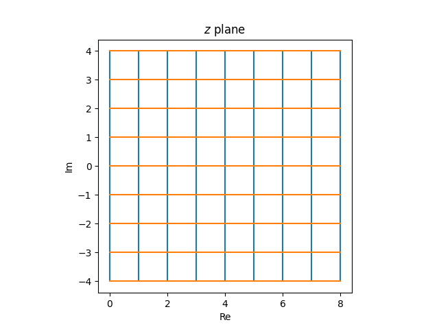
The Smith chart from electrical engineering is the picture of a Cartesian grid beneath the perform
f(z) = (z − 1)/(z + 1).
Extra particularly, it’s the picture of a grid in the suitable half-plane.
This submit will derive the essential mathematical properties of this graph however won’t go into the purposes. Stated one other approach, I’ll clarify the way to make a Smith chart, not the way to use one.
We’ll use z to indicate factors in the suitable half-plane and w to indicate the picture of those factors beneath f. We’ll converse of strains within the z airplane and the circles they correspond to within the w airplane.
Möbius transformations
Our perform f is a particular case of a Möbius transformation. There’s a theorem that claims Möbius transformation map generalized circles to generalized circles. Right here a generalized circle means a circle or a line; you’ll be able to consider a line as a circle with infinite radius. We’re going to get loads of mileage out of that theorem.
Picture of the imaginary axis
The perform f maps the imaginary axis within the z airplane to the unit circle within the w airplane. We are able to show this utilizing the theory above. The imaginary axis is a line, so it’s picture is both a line or a circle. We are able to take three factors on the imaginary axis within the z airplane and see the place they go.
Once we decide z equal to 0, i, and −i from the imaginary axis we get w values of −1, i, and −i. These three w values don’t line on a line, so the picture of the imaginary axis have to be a circle. Moreover, three factors uniquely decide a circle, so the picture of the imaginary axis is the circle containing −1, i, and −i, i.e. the unit circle.
Picture of the suitable half-plane
The imaginary axis is the boundary of the suitable half-plane. Since it’s mapped to the unit circle, the suitable half-plane is both mapped to the inside of the unit circle or the outside of the unit circle. The purpose z = 1 goes to w = 0, and so the suitable half-plane is mapped contained in the unit circle.
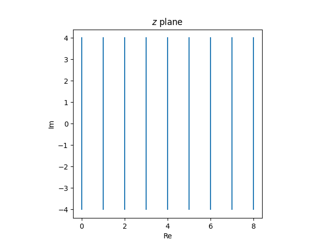
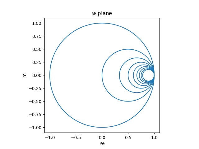
Pictures of vertical strains
Let’s take into consideration what occurs to vertical strains within the z airplane, strains with fixed constructive actual half. The pictures of those strains within the w airplane have to be both strains or circles. And because the right-half airplane will get mapped contained in the unit circle, these strains should get mapped to circles.
We are able to say somewhat extra. All strains comprise the purpose ∞, and f(∞) = 1, so the picture of each vertical line within the z airplane is a circle within the w airplane, contained in the unit circle and tangent to the unit circle at w = 1. (Tossing round ∞ is a bit casual, however it’s straightforward to make rigorous.)
The vertical strains within the z airplane
map to tangent circles within the w airplane.
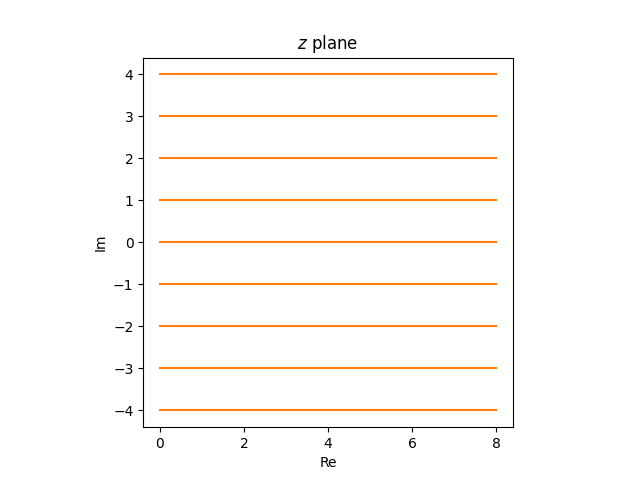
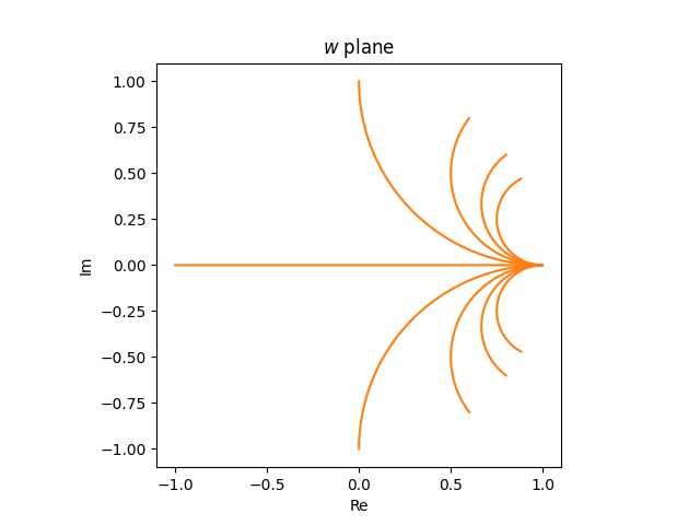
Pictures of horizontal strains
Subsequent, let’s take into consideration horizontal strains within the z airplane, strains with fixed imaginary half. The picture of those strains is both a line or a circle. Which is it? The picture of a line is a line if it accommodates ∞, in any other case it’s a circle. Now f(z) = ∞ if and provided that z = −1, and so the picture of the true axis is a line, however the picture of each different horizontal line is a circle.
Since f(∞) = 1, the picture of each horizontal line passes by 1, simply as the photographs of all of the vertical strains passes by 1.
Since horizontal strains lengthen previous the suitable half-plane, the picture circles lengthen previous the unit circle. The a part of the road with constructive actual half will get mapped contained in the unit circle, and the a part of the road with detrimental actual half will get mapped exterior the unit circle. Specifically, the picture of the constructive actual axis is the interval [−1, 1].
Möbius transformations are conformal maps, and they also protect angles of intersection. Since horizontal strains are perpendicular to vertical strains, the circles which can be the photographs of the horizontal strains meet the circles which can be the photographs of vertical strains at proper angles.
The horizontal rays within the z airplane
turn out to be partial circles within the w airplane.
If we have been to have a look at horizontal strains reasonably than rays, i.e. if we prolonged the strains into the left half-plane, the photographs within the w airplane could be full circles.
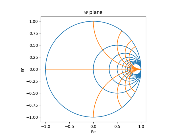
Now let’s put our photos collectively. The grid
within the z airplane turns into the next within the w airplane.
An evenly spaced grid within the z airplane turns into a really inconsistently spaced graph within the w airplane. Issues are crowded on the suitable hand aspect and sparse on the left. A useable Smith chart must be roughly evenly crammed in, which implies it must be the picture of an inconsistently crammed in grid within the z airplane. For instance, you’d want extra vertical strains within the z airplane with small actual values than with giant actual values.
The journey started in 1912 when Alexis Alexeieff launched a brand new genus for sure amoeboid kinds. He named it Naegleria in honor of Nägler’s analysis on amoebae that endure a biflagellate stage.
The particular pathogen liable for PAM, Naegleria fowleri, was first recognized in 1965 by Malcolm Fowler and Rodney F. Carter in Australia. They recorded the primary human circumstances, highlighting the lethal nature of the an infection.
In 1970, additional analysis utilizing mice helped isolate the pathogen, and it was formally named Naegleria fowleri in honor of Fowler, who recognized the illness from human mind tissue samples.
Milestones
The time period ‘major amoebic meningoencephalitis’ was coined in 1966 by Butt to tell apart this an infection from different sorts of meningoencephalitis.
Through the years, developments in diagnostic instruments have considerably improved our means to detect and perceive PAM. Amoeba cultures cerebrospinal fluid (CSF) and advances in molecular diagnostics, corresponding to polymerase chain response (PCR), immunofluorescence, and enzyme-linked immunosorbent assay (ELISA) enhanced the pace and accuracy of prognosis.
Imaging strategies like CT and MRI scans additionally play an important position in assessing the extent of mind harm.
Cultural influence and consciousness
Naegleria fowleri has not been related to any Nobel Prizes or landmark achievements in drugs, and little has been recognized about it for a very long time.
Nevertheless, this brain-eating amoeba was featured in an episode of the well-known American medical drama ‘Home M.D.,’ which elevated public consciousness of mind an infection and highlighted the damaging nature of the an infection.
As a teaser for our upcoming (2024-07-23) digital studying group session on Bayesian macro / time collection econometrics, this put up replicates a basic paper by Sims & Uhlig (1991) contrasting Bayesian and Frequentist inferences for a unit root. Within the put up I’ll give attention to explaining and implementing the authors’ simulation design. Within the studying group session (and presumably a future put up) we’ll discuss extra concerning the paper’s implications for the Bayesian-Frequentist debate and relate it to more moderen work by Mueller & Norets (2016). We’ll even be joined by particular visitor Frank Schorfheide who will assist information us by the current literature on Bayesian approaches to VARs, together with Giannone et al (2015) and (2019). Should you’re an Oxford scholar or workers member, you may join the studying group right here. In any other case, ship me an electronic mail and I’ll add you manually.
A Easy Instance
To set the stage for Sims & Uhlig (1991), think about the next easy instance: (X_1, X_2, dots X_{100} sim textual content{Regular}(mu, sigma^2)) the place (mu) is unknown however (sigma) is understood to equal (1). Let (bar{X} = frac{1}{100} sum_{i=1}^{100} X_i) be the pattern imply. Then (bar{X} pm 0.2) is an approximate 95% Frequentist confidence interval for (mu). In phrases: amongst 95% of the potential datasets that we might doubtlessly observe, the interval (bar{X} pm 0.2) will cowl the true, unknown worth of (mu); within the remaining (5%) of datasets, the interval won’t cowl (mu).
The Frequentist interval circumstances on (mu) and treats (bar{X}) as random. In distinction, a Bayesian credible interval circumstances on (bar{X}) and treats (mu) as random. This doesn’t require us to consider that (mu) is “actually” random. Bayesian reasoning merely makes use of the language of likelihood to precise uncertainty about any amount that we can’t observe. Let (bar{x}) be the noticed worth of (bar{X}). Beneath a obscure prior for (mu), e.g. a Regular(0, 100) distribution, the 95% Bayesian highest posterior density interval for (mu) is roughly (bar{x} pm 0.2). In phrases: on condition that we have now noticed (bar{X} = bar{x}), there’s a 95% likelihood that (mu) lies within the interval (bar{x} pm 0.2).
The comforting factor about this instance is that, no matter whether or not we select a Bayesian or Frequentist perspective, our inference stays the identical: compute the pattern imply, then add and subtract (0.2). Because of this the Frequentist interval inherits all the great properties of Bayesian inferences, and the Bayesian interval has appropriate Frequentist protection. This equivalence between Bayesian and Frequentist strategies crops up in lots of easy examples, particularly in conditions the place the pattern dimension is giant. However in additional advanced settings, the 2 approaches may give radically completely different solutions. And to move off a standard mis-understanding, this isn’t as a result of Bayesians use priors. Within the restrict as we accumulate increasingly more knowledge, the affect of the prior wanes. The important thing distinction is that Bayesian inference adheres to the chance precept, whereas frequent Frequentist strategies don’t.
A Not-so-simple Instance
Sims & Uhlig think about the AR(1) mannequin [
y_t = rho y_{t-1} + varepsilon_t, quad varepsilon_t sim text{iid Normal}(0, 1)
]
and the conditional most chance estimator given the preliminary (y_0), specifically [
widehat{rho} = frac{sum_{t=1}^T y_{t-1} y_t}{sum_{t=1}^T y_{t-1}^2}.
]
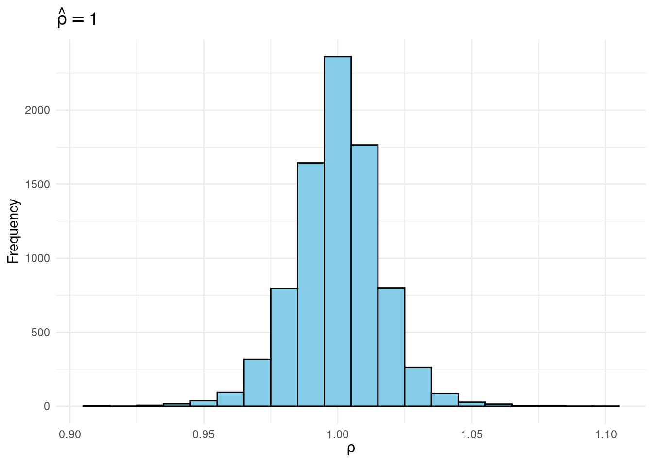
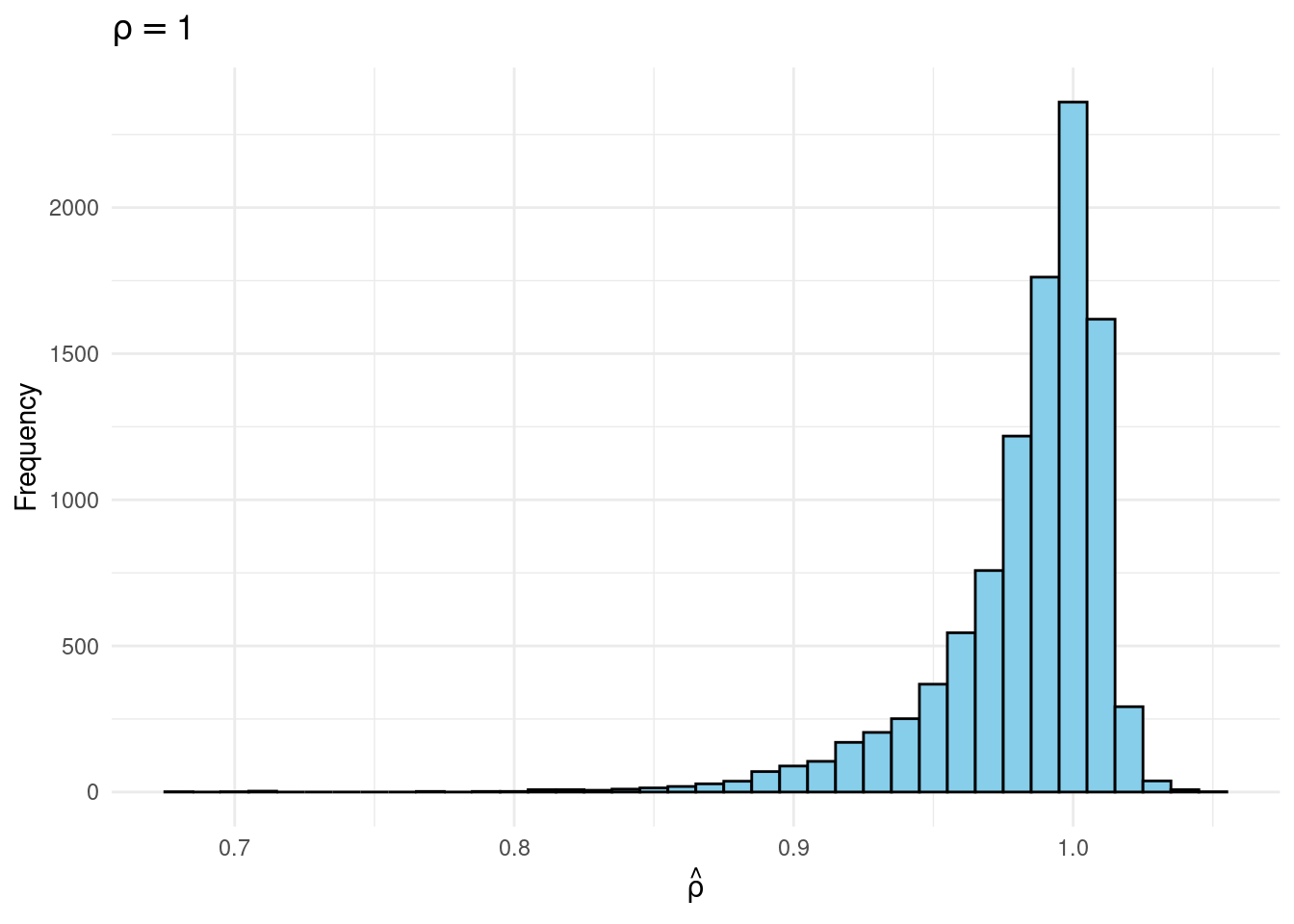
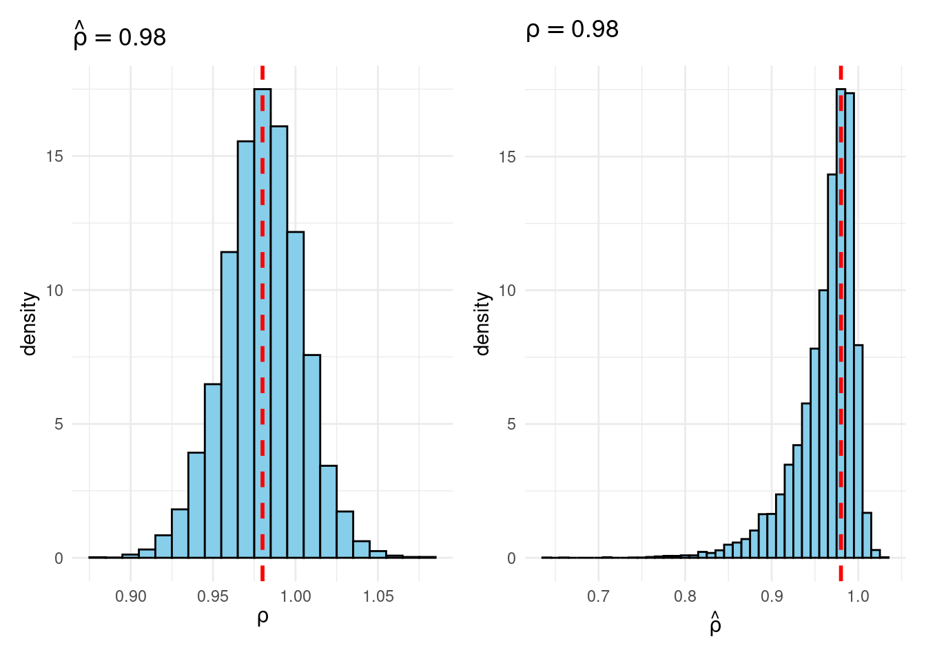
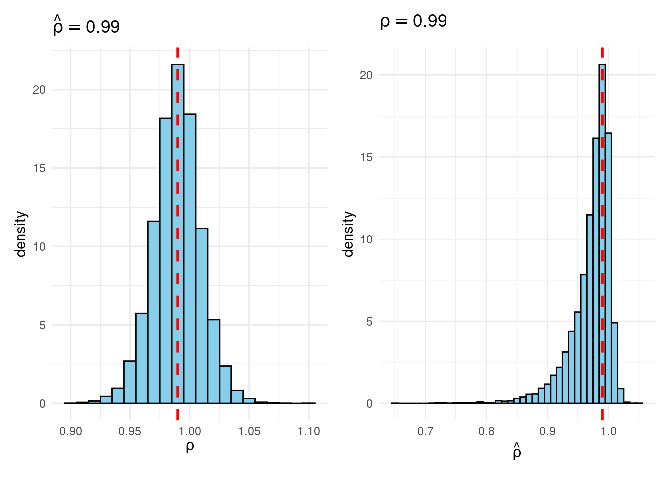
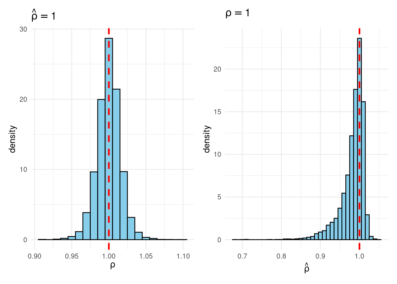
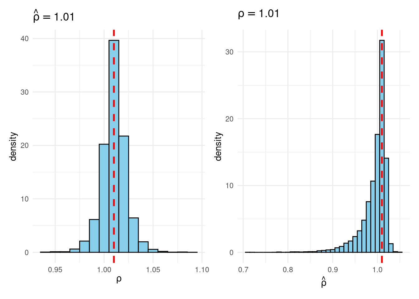
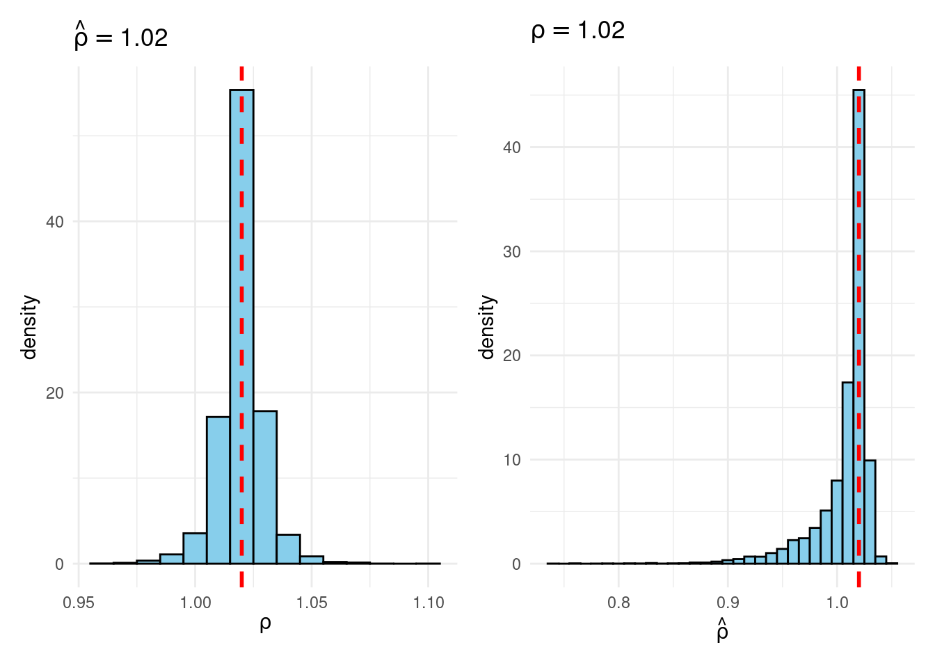
Their simulation contrasts the Frequentist sampling distribution of (widehat{rho}|rho) with the Bayesian posterior distribution of (rho|widehat{rho}) below a flat prior on (rho). When (rho) is close to one, these two distributions differ markedly: whereas the Bayesian posterior is all the time symmetric and centered at (widehat{rho} = widehat{rho}), the Frequentist sampling distribution is very skewed when (rho) is shut to 1. This exhibits that the Bayesian-Frequentist equivalence we present in our easy inhabitants imply instance from above breaks down fully on this extra advanced instance.
Sims & Uhlig argue that the Bayesian posterior gives a way more smart and helpful characterization of the knowledge contained within the knowledge and after studying the paper, I’m inclined to agree. My replication code follows under, together with plots of the joint distribution of ((rho, widehat{rho})) below a uniform prior for (rho) and the conditional distributions (widehat{rho}|rho=1) (Frequentist Sampling Distribution) and (rho|widehat{rho} = 1) (Bayesian Posterior).
The Replication
#-------------------------------------------------------------------------------
# Sims, C. A., & Uhlig, H. (1991). Understanding unit rooters: A helicopter tour
#
# (See additionally: Instance 6.10.6 from Poirier "Intermediate Statistics and 'Metrics")
#-------------------------------------------------------------------------------
# Within the subsequent part we are going to proceed to assemble, by Monte Carlo, an estimated
# joint pdf for rho and hat{rho} below a uniform prior pdf on rho. We select
# 31 values of rho, from 0.8 to 1.1 at intervals of 0.01. We draw 10000 100 x 1
# iid N(0,1) vectors of random variables to make use of a realizations of epsilon. For
# every of the 10000 epsilon vectors and every of the 31 rho values, we
# assemble a y vector with y(0) = 0, y(t) generated by equation (1).
#
# Equation (1): y(t) = rho y(t-1) + epsilon(t), t = 0, ..., T
#
# For every of those y vectors, we assemble hat{rho}. Utilizing as bins the
# intervals [-infty, 0.795), [0.795, 0.805), [0.805, 0.815), etc. we construct
# a histogram that estimates the pdf of hat{rho} for each fixed rho value.
# When these histograms are lined up side by side, they form a surface that is
# the joint pdf for rho and hat{rho} under a flat prior on rho.
#-------------------------------------------------------------------------------
set.seed(1693)

library(tidyverse)
library(tictoc)
library(patchwork)

draw_rho_hat <- function(rho) {
# Carry out the simulation once for a fixed value of rho; return rho_hat
  nT <- 100
  y <- rep(0, nT + 1)
  for (t in 2:(nT + 1)) {
    y[t] <- rho * y[t - 1] + rnorm(1)
  }
  y_t <- y[-1]
  y_tminus1 <- y[-length(y)]
  sum(y_t * y_tminus1) / sum(y_tminus1^2)
}

# Operate to run the simulation for a hard and fast worth of rho (10000 occasions)
run_sim <- (rho) map_dbl(1:1e4, (i) draw_rho_hat(rho))

tic()
foo <- run_sim(0.9)
toc() # ~0.6 seconds on my machine
## 0.595 sec elapsed
# Full sequence of rho values from Sims & Uhlig (1991)
rho <- seq(from = 0.8, to = 1.1, by = 0.01)

tic()
outcomes <- tibble(rho = rho,
                  rho_hat = map(rho, run_sim)) # Listing columns
toc() # ~17 seconds on my machine (1991 was a very long time in the past!)
## 16.814 sec elapsed
# The outcomes tibble makes use of a listing column for rho_hat. That is handy for
# making histograms of the frequentist sampling distribution (rho fastened) however
# not for making histograms of the Bayesian posterior (rho_hat) fastened. For the
# latter, we are going to use the unnest() perform to "develop" the checklist column rho_hat
# into a daily column. That is the "joint" distribution of rho and rho_hat.
joint <- outcomes |>
  unnest(rho_hat)

joint |>
  ggplot(aes(x = rho, y = rho_hat)) +
  geom_density2d_filled() +
  coord_cartesian(ylim = c(0.8, 1.1)) + # Prohibit rho_hat axis
  labs(title = "Joint Distribution",
       x = expression(rho),
       y = expression(hat(rho))) +
  theme_minimal()
# Operate that makes the previous two plots, places them side-by-side and lets
# the person specify the worth of rho/rho_hat that we situation on:
plot_Bayes_vs_Freq <- (r) >
    ggplot(aes(x = rho_hat)) +
    geom_histogram(aes(y = after_stat(density)),
                   binwidth = 0.01, fill = "skyblue", coloration = "black") +
    geom_vline(xintercept = r, coloration = "purple", linetype = "dashed", linewidth = 1) +
    labs(title = bquote(rho == .(spherical(r, 3))),
         x = expression(hat(rho))) +
    theme_minimal()

  p1 + p2


plot_Bayes_vs_Freq(0.98)