Saturday, January 24, 2026
Home Blog Page 211

How Composers Make Horror Film Music Sound Terrifying

0


The enduring bathe scene in Psycho was initially presupposed to play out with out music. As a substitute composer Bernard Herrmann created “The Homicide”: because the killing transpires, violins shriek and scream together with the sufferer.

The movie’s director, Alfred Hitchcock, reportedly later mentioned that “33 p.c of the impact of Psycho was because of the music.” In most horror flicks, the emotional present that carries the viewers is the music, which accelerates their anticipation and heightens the leap scares. It’s not simply screaming violins, both: undulating synthesizers drive John Carpenter’s Halloween;evil” clarinets underpin Hereditary; a recording from the Thirties enhances Get Out.

Research have proven that sure fearful music prompts the mind’s alarm-response system. So what’s it that makes some music sound scary? Psychoacoustics researchers have discovered that some auditory options which might be frequent in horror music are inherently scary. The obvious means music can scare us is by actually imitating screams, like Psycho does. Right here, the devices mimic a top quality of human screams known as roughness. Once we scream, we press a excessive quantity of air by our vocal cords, inflicting them to vibrate chaotically. This creates a sound wave with an amplitude that fluctuates quickly, which our ears and brains understand as tough or harsh.


On supporting science journalism

In case you’re having fun with this text, contemplate supporting our award-winning journalism by subscribing. By buying a subscription you’re serving to to make sure the way forward for impactful tales concerning the discoveries and concepts shaping our world right this moment.


To mimic this musically, violinists should push the boundaries of their devices. “They’re pushing into that string, actually—simply pushing the capability of the instrument. You’re feeling the entire instrument nearly resisting the sound,” explains Caitlyn Trevor, a music cognition researcher and founding father of the sound design consulting firm SonicUXR. In a 2020 research, when Trevor was a researcher on the College of Zurich, she and her colleagues studied horror film soundtracks and located many of those screamlike musical cues.

Tough vocalizations appear to have privileged entry to our mind. In a research printed in Might, scientists discovered that the sound of a distant scream might elicit a response from the mind even within the deepest stage of sleep. Whenever you hear a scream, it shortly prompts the amygdala, a mind construction concerned in processing hazard, and it will possibly set off a cascade of alarm reactions within the nervous system. The brief burst of sound might also set off our startle reflex, which bypasses higher-order mind areas and goes straight to our physique to assist us reply quick.

Most horror music will not be about immediately inducing terror, nonetheless. These moments of auditory launch are often preceded by lengthy, roiling tracks that construct suspense. “There are literally two very various kinds of music which might be ‘scary’ or ‘fearful,’” Trevor explains. In 2023 she co-authored a research analyzing the musical variations between these two sorts of horror film tracks. Contributors rated the emotional results of various excerpts. The outcomes confirmed a distinction between anxiety-inducing and terrifying music; the 2 sorts “generally have utterly reverse acoustic options,” Trevor says. The place terrifying music was loud, brash and dense (a refrain of screamlike string devices from Midsommar was ranked essentially the most terrifying of all of the examples within the research), anxiety-inducing music tended to be extra diverse. Right here is the place composers have essentially the most room to play, utilizing delicate auditory cues which might be biologically ingrained to maintain listeners on edge.

For instance, some horror motion pictures use (or are rumored to make use of) very low-frequency sounds on the border of human notion to provide an intangible sense of doom. “Sure sounds mimic hazard on the market on this planet,” explains Susan Rogers, a music producer and music cognition researcher at Berklee School of Music. “A low rumble is one thing we’ve developed to be alert to,” she says—maybe signaling a stampede, a storm, an earthquake or one thing else harmful within the setting.

Quick tempos, particularly ones that sound like a heartbeat, can even put us on edge, Rogers explains. Within the theme from John Carpenter’s Halloween, a low thudding that’s harking back to a heartbeat drives the music ahead. “A predictable rhythm offers you a way of momentum and that [the filmmakers are] main towards one thing,” Trevor says. The listener doesn’t know the place the music or the story are going, however they really feel relentless and inevitable.

Extra generally, although, horror film music builds suspense by making itself unpredictable. Suspenseful music, Trevor present in her 2023 research, typically retains us on edge by sprinkling in bits of sound in surprising locations. Typically these scores use an unpredictable or lopsided beat, dropping notes right here and there, to stop the listener from settling into the rhythm, she provides.

“The soundtrack and the sound design are integral to letting you are expecting what’s going to occur, so sound designers in horror motion pictures can use the strategy of violating our predictions to get us to expertise concern,” Rogers says. The mind is a prediction machine, and it permits us to tune out anticipated or fixed noise. “Whether or not it’s a automobile engine or a rainstorm, we all know the way it’s going to go, so we transfer our highlight of consideration onto different issues,” she continues. In case you hear footsteps arising the steps, you would possibly predict that they’ll proceed till they attain the highest; but when they cease midway, you turn out to be alert. These kinds of “prediction errors” activate the amygdala and a memory-forming area known as the hippocampus.

However among the most scary options of horror film music are culturally discovered and may not be inherently scary. For instance, composers typically construct stress in music utilizing dissonance, when the pitches of two or extra notes appear to conflict towards each other. The concept some harmonies are inherently dissonant has some reality—if two notes are too shut collectively in pitch, the soundwaves can intrude, inflicting a “beating” sample that may be disagreeable or grating on the ear. “However solely on the most simple stage is that common. Above that, the musical idea of consonance and dissonance is completely discovered,” Rogers says.

Different harmonies that had been as soon as assumed to be inherently dissonant—for instance, the so-called satan’s chord, or tritone, which is used typically in horror motion pictures—are perceived otherwise throughout completely different cultures. A 2016 research discovered that the Tsimane’ individuals of rural Bolivia, a bunch whose music doesn’t use concord, rated the tritone and different “dissonant” intervals as equally nice as “nondissonant” intervals.

Among the most inventive horror film soundtracks play on our cultural expectations to create a sense of unease or concern, Trevor provides. Many horror motion pictures make use of previous data, which have a warbling sound high quality and infrequently characteristic an old style means of singing that sounds odd to our trendy ears. This could create an uncanny valley impact—one thing that must be acquainted is as an alternative subtly unusual. “You realize what it’s, however there’s one thing fallacious with it,” Trevor says. “It’s not proper. And that’s actually disturbing at a deep stage.”

heatmaply: an R bundle for creating interactive cluster heatmaps for on-line publishing

0


What you should know

0


What are the primary indicators of RSV?

In response to the American Lung Affiliation (ALA), the preliminary indicators of RSV are just like delicate chilly signs and embrace:

  • Congestion
  • Runny nostril
  • Cough
  • Fever
  • Sore throat.

Very younger infants could have problem respiration and could also be irritable.

How lengthy does RSV final in kids?

The Cleveland Clinic notes that RSV often lasts between 3 to 7 days and that most individuals recuperate inside 2 weeks.

Are you able to get reinfected with RSV?

Sure, RSV reinfections are frequent.

Does RSV go away by itself?

Sure, most RSV infections go away on their very own, as per the US CDC. Nonetheless, in some instances, it could possibly trigger extreme respiratory signs.

Does Palivizumab forestall RSV?

Palivizumab is a monoclonal antibody medicine advisable to forestall respiratory syncytial virus (RSV) an infection in high-risk infants and youngsters.

Palivizumab binds to the virus and prevents it from infecting cells. It’s given as a month-to-month injection throughout the RSV season.

Whereas Palivizumab is efficient in lowering the chance of extreme an infection, it isn’t a assure and doesn’t present full safety.

Different preventive measures, such nearly as good hand hygiene and avoiding shut contact with sick people, also needs to be practiced to additional scale back the chance of RSV infections.

Can RSV be cured?

There isn’t a remedy for Respiratory Syncytial Virus (RSV), however generally, it causes delicate to reasonable cold-like signs and might be managed at residence.

Nonetheless, extra critical signs can happen in some instances, together with wheezing, extreme coughing suits, and problem respiration.

Preventive measures for individuals at a excessive danger of getting RSV embrace the RSV vaccine, Palivizumab antibody medicine, good hand hygiene, and avoiding shut contact with contaminated people.


Amassing Actual-Time Information with APIs: A Fingers-On Information Utilizing Python

0


Amassing Actual-Time Information with APIs: A Fingers-On Information Utilizing Python
Picture by Writer


Introduction

 
The flexibility to gather high-quality, related info continues to be a core talent for any information skilled. Whereas there are a number of methods to assemble information, probably the most highly effective and reliable strategies is thru APIs (utility programming interfaces). They function bridges, permitting completely different software program programs to speak and share information seamlessly.

On this article, we’ll break down the necessities of utilizing APIs for information assortment — why they matter, how they work, and methods to get began with them in Python.


What’s an API?

 
An API (utility programming interface) is a algorithm and protocols that permits completely different software program programs to speak and alternate information effectively.
Consider it like eating at a restaurant. As a substitute of talking on to the chef, you place your order with a waiter. The waiter checks if the elements can be found, passes the request to the kitchen, and brings your meal again as soon as it’s prepared.
An API works the identical manner: it receives your request for particular information, checks if that information exists, and returns it if out there — serving because the messenger between you and the information supply.
When utilizing an API, interactions usually contain the next parts:

  • Shopper: The appliance or system that sends a request to entry information or performance
  • Request: The shopper sends a structured request to the server, specifying what information it wants
  • Server: The system that processes the request and offers the requested information or performs an motion
  • Response: The server processes the request and sends again the information or end in a structured format, normally JSON or XML


Collecting Real-Time Data with APIs: A Hands-On Guide Using PythonCollecting Real-Time Data with APIs: A Hands-On Guide Using Python
Picture by Writer


This communication permits purposes to share info or functionalities effectively, enabling duties like fetching information from a database or interacting with third-party companies.


Why Utilizing APIs for Information Assortment?

 
APIs provide a number of benefits for information assortment:

  • Effectivity: They supply direct entry to information, eliminating the necessity for handbook information gathering
  • Actual-time Entry: APIs usually ship up-to-date info, which is important for time-sensitive analyses
  • Automation: They permit automated information retrieval processes, decreasing human intervention and potential errors
  • Scalability: APIs can deal with giant volumes of requests, making them appropriate for intensive information assortment duties


Implementing API Calls in Python

 
Making a primary API name in Python is without doubt one of the best and most sensible workouts to get began with information assortment. The favored requests library makes it easy to ship HTTP requests and deal with responses.
To show the way it works, we’ll use the Random Person Generator API, a free service that gives dummy consumer information in JSON format, excellent for testing and studying.
Right here’s a step-by-step information to creating your first API name in Python.


// Putting in the Requests Library:


// Importing the Required Libraries:

import requests
import pandas as pd


// Checking the Documentation Web page:

Earlier than making any requests, it is vital to know how the API works. This contains reviewing out there endpoints, parameters, and response construction. Begin by visiting the Random Person API documentation.


// Defining the API Endpoint and Parameters:

Primarily based on the documentation, we are able to assemble a easy request. On this instance, we fetch consumer information restricted to customers from america:

url="https://randomuser.me/api/"
params = {'nat': 'us'}


// Making the GET Request:

Use the requests.get() operate with the URL and parameters:

response = requests.get(url, params=params)


// Dealing with the Response:

Verify whether or not the request was profitable, then course of the information:

if response.status_code == 200:
    information = response.json()
    # Course of the information as wanted
else:
    print(f"Error: {response.status_code}")


// Changing Our Information right into a Dataframe:

To work with the information simply, we are able to convert it right into a pandas DataFrame:

information = response.json()
df = pd.json_normalize(information["results"])
df


Now, let’s exemplify it with an actual case. 


Working with the Eurostat API

 
Eurostat is the statistical workplace of the European Union. It offers high-quality, harmonized statistics on a variety of subjects reminiscent of economics, demographics, setting, trade, and tourism — masking all EU member states.

By means of its API, Eurostat affords public entry to an enormous assortment of datasets in machine-readable codecs, making it a priceless useful resource for information professionals, researchers, and builders occupied with analyzing European-level information.


// Step 0: Understanding the Information within the API:

If you happen to go verify the Information part of Eurostat, one can find a navigation tree. We are able to attempt to establish some information of curiosity within the following subsections:

  • Detailed Datasets: Full Eurostat information in multi-dimensional format
  • Chosen Datasets: Simplified datasets with fewer indicators, in 2–3 dimensions
  • EU Insurance policies: Information grouped by particular EU coverage areas
  • Cross-cutting: Thematic information compiled from a number of sources


// Step 1: Checking the Documentation:

At all times begin with the documentation. You will discover Eurostat’s API information right here. It explains the API construction, out there endpoints, and methods to kind legitimate requests.


Eurostat API base urlEurostat API base url


// Step 2: Producing the First Name Request:

To generate an API request utilizing Python, step one is putting in and importing the requests library. Keep in mind, we already put in it within the earlier easy instance. Then, we are able to simply generate a name request utilizing a demo dataset from the Eurostat documentation.

# We import the requests library
import requests

# Outline the URL endpoint -> We use the demo URL within the EUROSTATS API documentation.
url = "https://ec.europa.eu/eurostat/api/dissemination/statistics/1.0/information/DEMO_R_D3DENS?lang=EN"

# Make the GET request
response = requests.get(url)

# Print the standing code and response information
print(f"Standing Code: {response.status_code}")
print(response.json())  # Print the JSON response


Professional tip: We are able to cut up the URL into the bottom URL and parameters to make it simpler to perceive what information we are requesting from the API.

# We import the requests library
import requests

# Outline the URL endpoint -> We use the demo URL within the EUROSTATS API documentation.
url = "https://ec.europa.eu/eurostat/api/dissemination/statistics/1.0/information/DEMO_R_D3DENS"

# Outline the parameters -> We outline the parameters so as to add within the URL.
params = {
   'lang': 'EN'  # Specify the language as English
}

# Make the GET request
response = requests.get(url, params=params)

# Print the standing code and response information
print(f"Standing Code: {response.status_code}")
print(response.json())  # Print the JSON response


// Step 3: Figuring out Which Dataset to Name:

As a substitute of utilizing the demo dataset, you possibly can choose any dataset from the Eurostat database. For instance, let’s question the dataset TOUR_OCC_ARN2, which incorporates tourism lodging information.

# We import the requests library
import requests

# Outline the URL endpoint -> We use the demo URL within the EUROSTATS API documentation.
base_url = "https://ec.europa.eu/eurostat/api/dissemination/statistics/1.0/information/"
dataset = "TOUR_OCC_ARN2"

url = base_url + dataset
# Outline the parameters -> We outline the parameters so as to add within the URL.
params = {
    'lang': 'EN'  # Specify the language as English
}

# Make the GET request -> we generate the request and procure the response
response = requests.get(url, params=params)

# Print the standing code and response information
print(f"Standing Code: {response.status_code}")
print(response.json())  # Print the JSON response


// Step 4: Understanding the Response

Eurostat’s API returns information in JSON-stat format, a regular for multidimensional statistical information. It can save you the response to a file and discover its construction:

import requests
import json

# Outline the URL endpoint and dataset
base_url = "https://ec.europa.eu/eurostat/api/dissemination/statistics/1.0/information/"
dataset = "TOUR_OCC_ARN2"

url = base_url + dataset

# Outline the parameters so as to add within the URL
params = {
    'lang': 'EN',
    "time": 2019  # Specify the language as English
}

# Make the GET request and procure the response
response = requests.get(url, params=params)

# Verify the standing code and deal with the response
if response.status_code == 200:
    # Parse the JSON response
    information = response.json()

    # Generate a JSON file and write the response information into it
    with open("eurostat_response.json", "w") as json_file:
        json.dump(information, json_file, indent=4)  # Save JSON with fairly formatting

    print("JSON file 'eurostat_response.json' has been efficiently created.")
else:
    print(f"Error: Acquired standing code {response.status_code} from the API.")


// Step 5: Remodeling the Response into Usable Information:

Now that we acquired the information, we are able to discover a manner to put it aside right into a tabular format (CSV) to easy the method of analyzing it.

import requests
import pandas as pd

# Step 1: Make the GET request to the Eurostat API
base_url = "https://ec.europa.eu/eurostat/api/dissemination/statistics/1.0/information/"
dataset = "TOUR_OCC_ARN2"  # Vacationer lodging statistics dataset
url = base_url + dataset
params = {'lang': 'EN'}  # Request information in English

# Make the API request
response = requests.get(url, params=params)

# Step 2: Verify if the request was profitable
if response.status_code == 200:
    information = response.json()

    # Step 3: Extract the scale and metadata
    dimensions = information['dimension']
    dimension_order = information['id']  # ['geo', 'time', 'unit', 'indic', etc.]

    # Extract labels for every dimension dynamically
    dimension_labels = {dim: dimensions[dim]['category']['label'] for dim in dimension_order}

    # Step 4: Decide the scale of every dimension
    dimension_sizes = {dim: len(dimensions[dim]['category']['index']) for dim in dimension_order}

    # Step 5: Create a mapping for every index to its respective label
    # For instance, if we've got 'geo', 'time', 'unit', and 'indic', map every index to the proper label
    index_labels = {
        dim: record(dimension_labels[dim].keys())
        for dim in dimension_order
    }

    # Step 6: Create an inventory of rows for the CSV
    rows = []
    for key, worth in information['value'].objects():
        # `key` is a string like '123', we have to break it down into the corresponding labels
        index = int(key)  # Convert string index to integer

        # Calculate the indices for every dimension
        indices = {}
        for dim in reversed(dimension_order):
            dim_index = index % dimension_sizes[dim]
            indices[dim] = index_labels[dim][dim_index]
            index //= dimension_sizes[dim]

        # Assemble a row with labels from all dimensions
        row = {f"{dim.capitalize()} Code": indices[dim] for dim in dimension_order}
        row.replace({f"{dim.capitalize()} Title": dimension_labels[dim][indices[dim]] for dim in dimension_order})
        row["Value (Tourist Accommodations)"] = worth
        rows.append(row)

    # Step 7: Create a DataFrame and put it aside as CSV
    if rows:
        df = pd.DataFrame(rows)
        csv_filename = "eurostat_tourist_accommodation.csv"
        df.to_csv(csv_filename, index=False)
        print(f"CSV file '{csv_filename}' has been efficiently created.")
    else:
        print("No legitimate information to avoid wasting as CSV.")
else:
    print(f"Error: Acquired standing code {response.status_code} from the API.")


// Step 6: Producing a Particular View

Think about we simply need to maintain these information equivalent to Campings, Residences or Motels. We are able to generate a ultimate desk with this situation, and procure a pandas DataFrame we are able to work with.

# Verify the distinctive values within the 'Nace_r2 Title' column
set(df["Nace_r2 Name"])

# Record of choices to filter
choices = ['Camping grounds, recreational vehicle parks and trailer parks',
          'Holiday and other short-stay accommodation',
          'Hotels and similar accommodation']

# Filter the DataFrame based mostly on whether or not the 'Nace_r2 Title' column values are within the choices record
df = df[df["Nace_r2 Name"].isin(choices)]
df


Greatest Practices When Working with APIs


  • Learn the Docs: At all times verify the official API documentation to know endpoints and parameters
  • Deal with Errors: Use conditionals and logging to gracefully deal with failed requests
  • Respect Fee Limits: Keep away from overwhelming the server — verify if fee limits apply
  • Safe Credentials: If the API requires authentication, by no means expose your API keys in public code


Wrapping Up

 
Eurostat’s API is a robust gateway to a wealth of structured, high-quality European statistics. By studying methods to navigate its construction, question datasets, and interpret responses, you possibly can automate entry to crucial information for evaluation, analysis, or decision-making — proper out of your Python scripts.

You’ll be able to go verify the corresponding code in my GitHub repository My-Articles-Pleasant-Hyperlinks


Josep Ferrer is an analytics engineer from Barcelona. He graduated in physics engineering and is at present working within the information science area utilized to human mobility. He’s a part-time content material creator targeted on information science and know-how. Josep writes on all issues AI, masking the applying of the continuing explosion within the area.

OpenAI Releases Analysis Preview of ‘gpt-oss-safeguard’: Two Open-Weight Reasoning Fashions for Security Classification Duties


OpenAI has launched a analysis preview of gpt-oss-safeguard, two open weight security reasoning fashions that permit builders apply customized security insurance policies at inference time. The fashions are available two sizes, gpt-oss-safeguard-120b and gpt-oss-safeguard-20b, each positive tuned from gpt-oss, each licensed beneath Apache 2.0, and each accessible on Hugging Face for native use.

https://openai.com/index/introducing-gpt-oss-safeguard/

Why Coverage-Conditioned Security Issues?

Standard moderation fashions are skilled on a single mounted coverage. When that coverage modifications, the mannequin should be retrained or changed. gpt-oss-safeguard reverses this relationship. It takes the developer authored coverage as enter along with the person content material, then causes step-by-step to resolve whether or not the content material violates the coverage. This turns security right into a immediate and analysis process, which is best fitted to quick altering or area particular harms akin to fraud, biology, self hurt or sport particular abuse.

Similar Sample as OpenAI’s Inside Security Reasoner

OpenAI states that gpt-oss-safeguard is an open weight implementation of the Security Reasoner used internally throughout programs like GPT 5, ChatGPT Agent and Sora 2. In manufacturing settings OpenAI already runs small excessive recall filters first, then escalates unsure or delicate objects to a reasoning mannequin, and in current launches as much as 16 p.c of whole compute was spent on security reasoning. The open launch lets exterior groups reproduce this protection in depth sample as an alternative of guessing how OpenAI’s stack works.

Mannequin Sizes and {Hardware} Match

The big mannequin, gpt-oss-safeguard-120b, has 117B parameters with 5.1B energetic parameters and is sized to suit on a single 80GB H100 class GPU. The smaller gpt-oss-safeguard-20b has 21B parameters with 3.6B energetic parameters and targets decrease latency or smaller GPUs, together with 16GB setups. Each fashions had been skilled on the concord response format, so prompts should observe that construction in any other case outcomes will degrade. The license is Apache 2.0, the identical because the mother or father gpt-oss fashions, so business native deployment is permitted.

https://openai.com/index/introducing-gpt-oss-safeguard/

Analysis Outcomes

OpenAI evaluated the fashions on inside multi coverage exams and on public datasets. In multi coverage accuracy, the place the mannequin should accurately apply a number of insurance policies without delay, gpt-oss-safeguard and OpenAI’s inside Security Reasoner outperform gpt-5-thinking and the open gpt-oss baselines. On the 2022 moderation dataset the brand new fashions barely outperform each gpt-5-thinking and the inner Security Reasoner, nonetheless OpenAI specifies that this hole will not be statistically vital, so it shouldn’t be oversold. On ToxicChat, the inner Security Reasoner nonetheless leads, with gpt-oss-safeguard shut behind. This locations the open fashions within the aggressive vary for actual moderation duties.

OpenAI is express that pure reasoning on each request is pricey. The advisable setup is to run small, quick, excessive recall classifiers on all visitors, then ship solely unsure or delicate content material to gpt-oss-safeguard, and when person expertise requires quick responses, to run the reasoner asynchronously. This mirrors OpenAI’s personal manufacturing steering and displays the truth that devoted process particular classifiers can nonetheless win when there’s a massive prime quality labeled dataset.

Key Takeaways

  1. gpt-oss-safeguard is a analysis preview of two open weight security reasoning fashions, 120b and 20b, that classify content material utilizing developer provided insurance policies at inference time, so coverage modifications don’t require retraining.
  2. The fashions implement the identical Security Reasoner sample OpenAI makes use of internally throughout GPT 5, ChatGPT Agent and Sora 2, the place a primary quick filter routes solely dangerous or ambiguous content material to a slower reasoning mannequin.
  3. Each fashions are positive tuned from gpt-oss, hold the concord response format, and are sized for actual deployments, the 120b mannequin matches on a single H100 class GPU, the 20b mannequin targets 16GB stage {hardware}, and each are Apache 2.0 on Hugging Face.
  4. On inside multi coverage evaluations and on the 2022 moderation dataset, the safeguard fashions outperform gpt-5-thinking and the gpt-oss baselines, however OpenAI notes that the small margin over the inner Security Reasoner will not be statistically vital.
  5. OpenAI recommends utilizing these fashions in a layered moderation pipeline, along with neighborhood assets akin to ROOST, so platforms can categorical customized taxonomies, audit the chain of thought, and replace insurance policies with out touching weights.

OpenAI is taking an inside security sample and making it reproducible, which is a very powerful a part of this launch. The fashions are open weight, coverage conditioned and Apache 2.0, so platforms can lastly apply their very own taxonomies as an alternative of accepting mounted labels. The truth that gpt-oss-safeguard matches and typically barely exceeds the inner Security Reasoner on the 2022 moderation dataset, whereas outperforming gpt-5-thinking on multi coverage accuracy, however with a non statistically vital margin, exhibits the method is already usable. The advisable layered deployment is reasonable for manufacturing.


Michal Sutter is an information science skilled with a Grasp of Science in Information Science from the College of Padova. With a stable basis in statistical evaluation, machine studying, and information engineering, Michal excels at remodeling complicated datasets into actionable insights.

From JD Vance to Elon Musk, the proper loves The Lord of the Rings

0


Among the many many humiliations of being American within the present second is that this: Members of the tech proper and the conservative ruling class frequently fetishize objects of nerd tradition whereas additionally displaying a willful lack of ability to know the very primary messages these objects are sending. Whereas there are actually worse issues (e.g. white nationalism within the White Home), the blazing lack of studying comprehension from people who find themselves allegedly good does give one pause. Put merely, these persons are unhealthy nerds.

Most likely the textual content they’re most constantly vulnerable to misreading is The Lord of the Rings. J.R.R. Tolkien’s beloved fantasy trilogy offers with the corrupting affect of energy and the need of demise. But, the proper retains utilizing it as a parable for why highly effective individuals ought to be given extra energy and human beings ought to be immortal.

Most just lately, Elon Musk posted to his platform X that Tolkien’s peaceable hobbits have been capable of reside idyllic lives on the Shire solely as a result of “they have been protected by the arduous males of Gondor,” referring to the human kingdom entrenched in battle towards Mordor. England, Musk declared, should additionally ally with arduous males — on this case, the far proper anti-Islamic activist Tommy Robinson — to revive its personal peace and tranquility. Robinson is at present on trial within the UK, accused of refusing to adjust to counter-terrorism police and says Musk is paying his authorized payments.

Following Musk’s lead, the Division of Homeland Safety posted an ICE recruitment advert utilizing a screengrab of Merry (performed by Dominic Monaghan), one of many hobbits in Peter Jackson’s Lord of the Rings motion pictures. Superimposed over the picture is a line of Merry’s dialogue — “There received’t be a shire, pippin.” — after which, beneath it, the URL be a part of.ice.gov.

The thought right here is that the naive hobbits characterize the civilians of each the US and the UK, and unbeknownst to them, they’re being menaced by the forces of evil: Muslim migrants from the Center East, alleged to be invading each international locations. The one option to forestall it, the metaphor implies, is for the hobbits to ally with the “arduous males of Gondor” — Islamaphobic agitators for Musk and masked militias who assault unarmed civilians for the DHS — earlier than their lifestyle is gone utterly.

Nevertheless, you do not want to be a deep scholar of The Lord of the Rings — and buddies, I’m not one — to know that this metaphor utterly falls aside after a single step again.

In Tolkien’s books, it isn’t the lads of Gondor who flip again the forces of evil and save the Shire; it’s these mild, peaceable hobbits who pull the entire thing off. They’re the one species capable of carry the One Ring of Energy, as a result of they’re, by their nature, unambitious. All they need is to reside their peaceable bourgeois lives of tea and toast and jam, so they can stand up to the temptations of the ring and its guarantees of energy, in the end carrying it far sufficient to destroy it. The perfect the lads of Gondor can do to assist is refuse to ever contact the ring, as a result of they know that in the event that they decide it up, they won’t be able to withstand temptation.

To translate this into the metaphor: Should you’re taking Tolkien as your information, and also you imagine your homeland to be below invasion by the forces of evil, the answer is to not attempt to consolidate your energy, harden your nature, and glory in pointless cruelty. The answer is to refuse energy at any time when it’s supplied to you and to combat from a spot of humility.

The DHS and Musk aren’t the one members of the brand new proper to make use of Tolkien to justify their actions. As David French instructed As we speak, Defined earlier this fall, JD Vance has described The Lord of the Rings as elementary to his journey into conservatism, a lot in order that he named his enterprise capital agency Narya after considered one of Tolkien’s magic rings. Vance’s mentor Peter Thiel named his personal enterprise capital agency Mithril, after considered one of Tolkien’s magic metals. One other considered one of Thiel’s corporations — an AI platform Trump is utilizing to surveil and monitor Individuals — is called after Palantir, a magical artifact that the Lord of the Rings villain Sauron makes use of to observe and deceive the individuals of Center-earth.

The darkness of that parallel is kind of par for the course for Thiel, who constantly appears to empathize most with Tolkien’s villains. In a 2023 interview with the Atlantic, Thiel declared that he had learn the trilogy at the least 10 instances, and that he had come to the conclusion that the one distinction between Tolkien’s elves and his people is that the elves are immortal and don’t die. “Why can’t we be elves?” requested Thiel, who has spoken at size about his curiosity in extending his personal life, maybe to the purpose of immortality.

One of many recurring plots of The Lord of the Rings is in truth tales about human beings who attempt to be immortal just like the elves and are corrupted by that try, their lives ruined. They turn into undead or insane; they cling onto grotesque caricatures of life. Demise in these books is named The Present of Males. It’s what provides human lives their form and that means. Elves are naturally immortal, however people who attempt to be immortal are corrupted as certainly as those that thirst for energy. For Tolkien, mortality is a present, not one thing to be fled in terror.

None of those messages are obscure. They’re floor degree. Kids in center faculty repeatedly pull them out of those books with out issue. But, for some motive, a bunch of extremely highly effective males who satisfaction themselves on their very own intelligence and who additionally think about Tolkien’s philosophy to be elementary to their worldview appear to be having quite a lot of bother.

The Lord of the Rings really has a reasonably respectable metaphor for what occurs when highly effective individuals determine to willfully ignore the knowledge of individuals they declare to respect and conclude that the one means they are often of service to the world is by chasing energy for themselves. That’s what occurs to Saruman the wizard, and he finally ends up invading the Shire himself. The boys of Gondor don’t cease him in any respect.

Physicists Simply Dominated Out The Universe Being a Simulation : ScienceAlert

0


A query that has vexed physicists for the previous century might lastly have an answer – however maybe not the one everybody hoped for.

In a brand new, detailed breakdown of present idea, a crew of physicists led by Mir Faizal of the College of British Columbia has proven that there isn’t a common “Idea of All the things” that neatly reconciles normal relativity with quantum mechanics – not less than, not an algorithmic one.

A pure consequence of that is that the Universe cannot be a simulation, since any such simulations must function algorithmically.

Associated: Slime Mould Has Been Used to Recreate The Invisible Internet Holding Our Universe Collectively

“We’ve demonstrated that it’s unattainable to explain all facets of bodily actuality utilizing a computational idea of quantum gravity,” Faizal says.

“Due to this fact, no bodily full and constant idea of every little thing may be derived from computation alone. Relatively, it requires a non-algorithmic understanding, which is extra elementary than the computational legal guidelines of quantum gravity and due to this fact extra elementary than spacetime itself.”

Some of the pernicious thorns in our understanding of how every little thing works is the insoluble relationship between the seamless cloth of spacetime and the fuzzy duality of quantum mechanics. We all know that the Universe does operate, however the arithmetic used to explain every realm collapses when utilized to the opposite.

Physicists have lengthy sought a mathematical answer – a so-called quantum gravity, or Idea of All the things – that may permit physics to easily transition between normal relativity and quantum idea.

Faizal and his colleagues highlighted in style makes an attempt to resolve issues with this transition, like string idea and loop quantum gravity.

These suggest spacetime and quantum fields emerge from a basis of pure data, past which nothing exists – described succinctly by American theoretical physicist John Wheeler as getting an “it from a bit“.

But there are good causes, the crew says, that “its” cannot come from “bits”.

frameborder=”0″ permit=”accelerometer; autoplay; clipboard-write; encrypted-media; gyroscope; picture-in-picture; web-share” referrerpolicy=”strict-origin-when-cross-origin” allowfullscreen>

“Drawing on mathematical theorems associated to incompleteness and indefinability, we exhibit {that a} absolutely constant and full description of actuality can’t be achieved by means of computation alone,” Faizal explains.

“It requires non-algorithmic understanding, which by definition is past algorithmic computation and due to this fact can’t be simulated. Therefore, this Universe can’t be a simulation.”

Arguing that the data from which actuality emerges would must be each elementary and finite, the physicists turned to mathematicians Kurt Gödel, Alfred Tarski, and Gregory Chaitin to interrogate their speculation.

These three theoreticians – the latter two working within the first half of the twentieth century, and Chaitin from the Nineteen Sixties – independently confirmed that there are arduous limits to our potential to grasp the Universe.

Gödel’s well-known 1931 incompleteness theorems confirmed that any constant mathematical system will include true statements that however can’t be confirmed utilizing its personal guidelines. Tarski’s 1933 undefinability theorem confirmed that an arithmetical system can’t outline its personal reality.

Lastly, Chaitin’s incompleteness theorem – which is analogous to Gödel’s work – exhibits that there is a arduous higher restrict to how a lot complexity a proper algorithmic system can describe.

Utilizing these logical theorems, the researchers discover that physics itself can’t be absolutely computable. They suggest that the one solution to resolve a Idea of All the things is so as to add a non-algorithmic layer above the algorithmic one to create a Meta Idea of All the things, or MToE.

Win a $10,000 Space Coast Adventure Holiday

This meta-layer would be capable to decide what’s true from outdoors the mathematical system, giving scientists a solution to examine phenomena such because the black gap data paradox with out violating mathematical guidelines.

And, after all, it places to mattress that pesky drawback of whether or not we’re really “actual”.

“Any simulation is inherently algorithmic – it should comply with programmed guidelines,” Faizal says. “However for the reason that elementary stage of actuality is predicated on non-algorithmic understanding, the universe can’t be, and will by no means be, a simulation.”

The analysis has been printed within the Journal of Holography Functions in Physics.

AI Success, However Not Enterprise Success

0


Of their guide, “Mining Your Personal Enterprise,” Jeff Deal and Gerhard Pilcher, COO and CEO of Elder Analysis respectively, describe what I’ll name “The Case of the Climbing Churn.” Churn is when a subscriber cancels or fails to resume a service or subscription. A profitable predictive mannequin for figuring out probably churners was deployed for a cell phone service supplier, and name heart brokers started reaching out to them to encourage renewals. Sadly, the churn fee rose!

Anybody trying to achieve one other get together on the telephone is aware of that the most definitely final result is failure to reply the telephone. Investigation revealed that in these many circumstances of non-reply, the brokers had been leaving voicemail messages for the shoppers. These voicemails, as an alternative of producing renewals, had been alerting subscribers that their contracts had been about to run out, successfully letting them know that they may now change carriers with out penalty.

Fixing the issue was straightforward, requiring solely a level of enterprise sense: brokers had been informed to not depart voicemails. Churn then dropped, as predicted by the mannequin, since many purchasers discovered the renewal affords after they may very well be defined, interesting. The churn discount from utilizing the mannequin the best approach for only one month greater than paid for its growth; after that, it was all revenue.

Subsequent, we flip to a few circumstances the place strategic actions or inactions, unrelated to AI, dampened the enterprise trajectory of a few well-known companies that had been constructed on information and machine studying.

PANDORA

Pandora is an web music radio service primarily based absolutely on predictive algorithms and information. It permits customers to construct personalized “stations” that play music much like a tune or artist that they’ve specified. When it began, Pandora used a nearest-neighbor model clustering/classification course of referred to as the Music Genome Mission to find new songs or artists like a user-specified tune or artist.

Pandora was the brainchild of Tim Westergren, who labored as a musician and a nanny when he graduated from Stanford within the Nineteen Eighties. Along with Nolan Gasser, who was finding out medieval music, he developed a “matching engine” by getting into information a couple of tune’s traits right into a spreadsheet.

In simplified phrases, the method labored roughly as follows for songs:

Pandora established tons of of variables on which a tune will be measured on a scale from 0 to five. 4 such variables from the start of the checklist are:

●Acid Rock Qualities
●Accordion Enjoying
●Acousti – Lectric Sonority
●Acousti -Artificial Sonority 

Pandora paid musicians to fee tens of hundreds of songs on every of those attributes. This step represented a major funding and supplied a foundation for outlining extremely individualized preferences as a consumer gave a thumbs up or thumbs down whereas listening. Over time, Pandora developed the flexibility to ship songs that matched the style of every consumer. A single consumer may construct up a number of stations round totally different tune clusters. Clearly, this can be a extra refined strategy than choosing music on the idea of which “style” it belongs to.

Observe the function of area data on this machine studying course of. The variables had been examined and chosen by the undertaking leaders, and the measurements had been made by human consultants. But, this human function was the Achilles heel of Pandora: it was a pricey bottleneck, obstructing the stream of recent songs into the system.

Because the business matured, music streaming providers later got here to omit this step of pre-labeling songs, and to depend on machine studying algorithms that get enter solely from customers. Collaborative filtering, for instance, recommends songs which are appreciated by different individuals who share your tastes (take pleasure in the identical songs). Deep studying networks (which weren’t virtually out there at Pandora’s inception) can take the sound waves in songs and derive options that may then be used to foretell consumer selections.

Pandora was a pioneer in licensed music streaming however was later eclipsed by Spotify and Apple Music. The important thing aggressive differentiator between Pandora and its rivals, although, was not a distinction in algorithms. The truth is, it had nothing to do with AI. Relatively, it was the character of the product being offered. Pandora was designed to be “customized radio.” It didn’t allow you to play songs on-demand or construct up a library of downloaded music. Spotify and Apple Music each provide these options to customers, which gave them a leg up within the market. They now declare greater than half the worldwide market, with Pandora diminished to 2%.

AI Success, However Not Enterprise Success

supply: https://www.t4.ai/business/music-streaming-market-share

To be honest, Pandora’s future was hobbled by the previous from which it emerged. The business music enterprise had efficiently fought off challenges from web platforms like Napster, the place customers might broadly redistribute songs with out paying royalties. Pandora determined to create a authentic streaming path, however its enterprise mannequin couldn’t afford to pay artists royalties akin to these paid by file firms. Its mission was, subsequently, circumscribed from the start to keep away from authorized challenges from the music business. In establishing itself as an early market chief, Pandora softened up the music business to the purpose the place it accepted the inevitability of streaming, opening the way in which for rivals to supply extra to the shopper.

ZILLOW

The web is known for disrupting present companies, and, in 2004, the house sale enterprise represented one of many largest targets. Over 3 million realtors within the U.S. loved a cartel-like safety from competitors within the type of “ethics” codes that dictated adherence to a strict fee construction. Promulgated and promoted by realtor organizations, the codes successfully assured a fee within the neighborhood of 6%. The business was extraordinarily disaggregated, with no brokerage firm accounting for greater than 3% of the realtor brokers.

In 2004 Zillow arrived with an web platform that allowed householders and potential purchasers to see the estimated worth of just about any home they had been fascinated by. This data was beforehand the province of licensed realtors by way of the A number of Itemizing Service. Zillow went public in 2011. Its statistical fashions on which worth estimates had been primarily based didn’t require data that was onerous to seek out, and, certainly, relied closely on assessed values of properties, which had been publicly out there. The mechanics and energy required to acquire these information constituted the majority of the modeling effort. However, even when lower than 100% correct, the estimates attracted shopper consideration and, as soon as they grew to become ubiquitous, the Zillow platform grew to become a pretty place for realtors to promote. Because the platform grew to become extra dominant and broadly used, the necessity for realtors to be seen on Zillow elevated, and the promoting premium that Zillow might command grew. Zillow’s technique was to simply accept the function of unbiased realtors however seize increasingly of the fee within the type of advert charges.

Zillow’s place was challenged by one other web entrant, Redfin, which supplied an analogous platform that enabled shoppers to view home costs. Not like Zillow, Redfin didn’t eschew the realtor function itself -in reality, it began enterprise as an actual property brokerage. Redfin sells houses on to shoppers through its personal brokers, posing extra of a problem to the established business. By providing this extra conventional gross sales service, a service unrelated to predictive algorithms, Redfin started to catch as much as Zillow. The 2 are actually roughly equal in market.

Conclusion:

Zillow, whose inventory worth was flagging within the a number of years previous to 2020, has been revitalized by the robust housing market that adopted the tip of pandemic lockdowns. The corporate is now doing properly, typical realty brokerages proceed to promote with it, and it stays an open query whether or not a “information + promoting” technique (Zillow) or a “information + gross sales drive” technique (Redfin) will prevail. Or, maybe, a 3rd competitor with a brand new technique will emerge: conventional unbiased realtors have continued as a robust drive and stay a goal for disruption.

Observe: In its consulting engagements, Elder Analysis is understood for growing analytics methods solely within the context of a broader enterprise technique. Learn extra in Main a Knowledge Analytics Initiative, an e book extract from Mining your Personal Enterprise.


Bayesian threshold autoregressive fashions – The Stata Weblog

0


Autoregressive (AR) fashions are a number of the most generally used fashions in utilized economics, amongst different disciplines, due to their generality and ease. Nonetheless, the dynamic traits of actual financial and monetary knowledge can change from one time interval to a different, limiting the applicability of linear time-series fashions. For instance, the change of unemployment charge is a perform of the state of the financial system, whether or not it’s increasing or contracting. A wide range of fashions have been developed that enable time-series dynamics to rely upon the regime of the system they’re a part of. The category of regime-dependent fashions embrace Markov-switching, easy transition, and threshold autoregressive (TAR) fashions.

TAR (Tong 1982) is a category of nonlinear time-series fashions with purposes in econometrics (Hansen 2011), monetary evaluation (Cao and Tsay 1992), and ecology (Tong 2011). TAR fashions enable regime-switching to be triggered by the noticed stage of an end result up to now. The threshold command in Stata gives frequentist estimation of some TAR fashions.

In Stata 17, the bayesmh command helps time-series operators in linear and nonlinear mannequin specs; see [BAYES] bayesmh. On this weblog entry, I wish to present how we will match some Bayesian TAR fashions utilizing the bayesmh command. The examples will even reveal modeling flexibility not doable with the present threshold command.

TAR mannequin definition

Let ({y_t}) be a collection noticed at discrete instances (t). A common TAR mannequin of order (p), TAR((p)), with (ok) regimes has the shape
[
y_t = a_0^{j} + a_1^{j} y_{t-1} + dots + a_p^{j} y_{t-p} + sigma_{j} e_t, quad {rm if} quad
r_{j-1} < z_t le r_{j}
]
the place (z_t) is a threshold variable, (-infty < r_0 < dots < r_k =
infty) are regime thresholds, and (e_t) are unbiased customary usually distributed errors. The (j)th regime has its personal set of autoregressive coefficients ({a_i^j})’s and customary deviations (sigma_j)’s. Totally different regimes are additionally allowed to have totally different orders (p). Within the above equation, this may be indicated by changing (p) with regime-specific (p_j)’s.

In a TAR mannequin, as implied by the definition, structural breaks occur not at sure time factors however are triggered by the magnitude of the brink variable (z_t). It is not uncommon to have (z_t = y_{t-d}), the place (d) is a constructive integer the referred to as the delay parameter. These fashions are referred to as self-exciting TAR (SETAR) and are those I’m illustrating under.

Actual GDP dataset

In Beaudry and Koop (1993), TAR fashions have been used to mannequin gross nationwide product. The authors demonstrated uneven persistence within the progress charge of gross nationwide product, with constructive shocks (related to enlargement durations) being extra persistent than detrimental shocks (recession durations). In an analogous method, I take advantage of the expansion charge of actual gross home product (GDP) of america as an indicator of the standing of the financial system to mannequin the distinction between enlargement and recession durations.

Quarterly observations on actual GDP, measured in billions of {dollars}, are obtained from the Federal Reserve Financial Knowledge repository utilizing the import fred command. I take into account observations solely between the primary quarter of 1947 and second quarter of 2021. A quarterly date variable, dateq, is generated and used with tsset to arrange the time collection.

. import fred GDPC1

Abstract
-------------------------------------------------------------------------------
Sequence ID                    Nobs    Date vary                Frequency
-------------------------------------------------------------------------------
GDPC1                        301     1947-01-01 to 2022-01-01  Quarterly
-------------------------------------------------------------------------------
# of collection imported: 1
   highest frequency: Quarterly
    lowest frequency: Quarterly

. maintain if daten >= date("01jan1947", "DMY") & daten <= 
> date("01apr2021", "DMY")
(3 observations deleted)

. generate dateq = qofd(daten)

. tsset dateq, quarterly

Time variable: dateq, 1947q1 to 2021q2
        Delta: 1 quarter

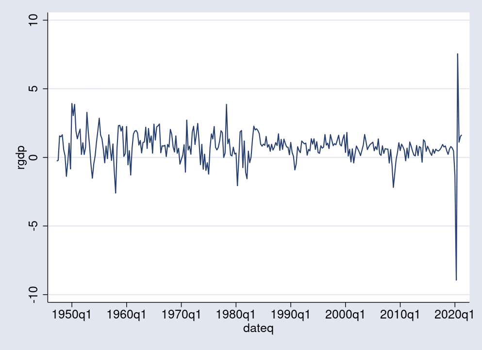
I’m within the change of actual GDP from one quarter to the following. For this function, I generate a brand new variable, rgdp, to measure this modification in percentages. Constructive values of rgdp point out financial progress or enlargement, whereas values near 0 or detrimental are related to stagnation or recession. Under, I take advantage of the tsline command to plot the time collection. There, a number of the recession durations, indicated by sharp drops in GDP, are seen, together with the most recent one in 2020.

. generate double rgdp = 100*D1.GDPC1/L1.GDPC1
(1 lacking worth generated)

. tsline rgdp

A TAR mannequin with two regimes estimates one threshold worth (r) that may be visualized as a horizontal line separating, considerably informally, enlargement from recession durations. In Bayesian TAR, the brink (r) is a random variable with distribution estimated from a previous and noticed knowledge.

Bayesian TAR specification

Earlier than I present how one can specify a Bayesian TAR mannequin in Stata, let me first match a less complicated Bayesian AR(1) mannequin for rgdp utilizing the bayesmh command. It can function a baseline for comparability with fashions with structural breaks.

I take advantage of the pretty uninformative, given the vary of rgdp, regular(0, 100) prior for the 2 coefficients within the {rgdp:} equation and the igamma(0.01, 0.01) prior for the variance parameter {sig2}. I additionally use Gibbs sampling for extra environment friendly simulation of the mannequin parameters.

. bayesmh rgdp L1.rgdp, chance(regular({sig2}))                
>         prior({rgdp:}, regular(0, 100)) block({rgdp:}, gibbs)    
>         prior({sig2}, igamma(0.01, 0.01)) block({sig2}, gibbs)  
>         rseed(17) dots

Burn-in 2500 .........1000.........2000..... carried out
Simulation 10000 .........1000.........2000.........3000.........4000.........
> 5000.........6000.........7000.........8000.........9000.........10000 carried out

Mannequin abstract
------------------------------------------------------------------------------
Probability:
  rgdp ~ regular(xb_rgdp,{sig2})

Priors:
  {rgdp:L.rgdp _cons} ~ regular(0,100)                                      (1)
               {sig2} ~ igamma(0.01,0.01)
------------------------------------------------------------------------------
(1) Parameters are parts of the linear kind xb_rgdp.

Bayesian regular regression                       MCMC iterations  =     12,500
Gibbs sampling                                   Burn-in          =      2,500
                                                 MCMC pattern dimension =     10,000
                                                 Variety of obs    =        296
                                                 Acceptance charge  =          1
                                                 Effectivity:  min =      .9584
                                                              avg =      .9755
Log marginal-likelihood = -478.07327                          max =          1

------------------------------------------------------------------------------
             |                                                Equal-tailed
             |      Imply   Std. dev.     MCSE     Median  [95% cred. interval]
-------------+----------------------------------------------------------------
rgdp         |
        rgdp |
         L1. |  .1239926   .0579035   .000591   .1240375   .0096098    .237592
             |
       _cons |  .6762768   .0805277   .000805    .676687   .5186598   .8378632
-------------+----------------------------------------------------------------
        sig2 |  1.344712   .1098713   .001117   1.339746   1.144444   1.571802
------------------------------------------------------------------------------

The posterior imply estimate for the AR(1) coefficient {L1.rgdp} is 0.12, indicating a constructive serial correlation for rgdp. This means a point of persistence in the true GDP progress. The posterior imply estimate of 1.34 for {sig2} suggests a volatility stage above 1 p.c, if the latter is measured by customary deviation. Nonetheless, this straightforward AR(1) mannequin doesn’t inform us how the persistence and volatility change relying on the state of the financial system.

Earlier than persevering with, I save the simulation and estimation outcomes for later reference.

. bayesmh, saving(bar1sim, substitute)
word: file bar1sim.dta saved.

. estimates retailer bar1

To explain a two-state mannequin for the financial system, I wish to specify the best two-regime SETAR mannequin with order of 1 and delay of 1. Within the subsequent part, I focus on the selection of order and delay parameters.

The mannequin may be summarized by the next two equations:
start{align}
{bf rgdp_t} = a_0^{1} + a_1^{1} {bf rgdp_{t-1}} + sigma_{1} e_t, quad {rm if} quad
y_{t-1} < r
{bf rgdp_t} = a_0^{2} + a_1^{2} {bf rgdp_{t-1}} + sigma_{2}
e_t, quad {rm if} quad y_{t-1} ge r
finish{align}

To specify the regression portion of this mannequin with bayesmh, I take advantage of a substitutable expression with conditional logic,

cond(L1.rgdp<{r}, {r1:a0}+{r1:a1}*L1.rgdp, {r2:a0}+{r2:a1}*L1.rgdp)

the place {r1:a0} and {r1:a1} are the coefficients for the primary regime and {r2:a0} and {r2:a1} are the coefficients for the second regime.

The regime-specific variance of the conventional chance may be equally
specified by the expression

cond(L1.rgdp<{r},{sig1},{sig2})

As an alternative of assuming a hard and fast threshold worth for (r), with 0 being a pure selection, I take into account (r) to be a hyperparameter with uniform(-0.5, 0.5) prior. I thus assume that the brink is inside a half proportion level of 0. Given the vary of rgdp and that 0 separates constructive from detrimental progress, this appears to be an affordable assumption. Utilizing uninformative priors for (r) with none restrictions on its vary will make the mannequin unstable due to the potential of collapsing one of many regimes, that’s, having a regime with 0 or only some noticed factors. The priors for coefficients and variances keep the identical as within the earlier mannequin.

. bayesmh rgdp = (cond(L1.rgdp<{r},                               
>                 {r1:a0}+{r1:a1}*L1.rgdp,                        
>                 {r2:a0}+{r2:a1}*L1.rgdp)),                      
>         chance(regular(cond(L1.rgdp<{r}, {sig1}, {sig2})))   
>         prior({r1:}, regular(0, 100)) block({r1:})               
>         prior({r2:}, regular(0, 100)) block({r2:})               
>         prior({sig1}, igamma(0.01, 0.01)) block({sig1})         
>         prior({sig2}, igamma(0.01, 0.01)) block({sig2})         
>         prior({r}, uniform(-0.5, 0.5)) block({r})               
>         rseed(17) init({sig1} {sig2} 1) dots

Burn-in 2500 aaaaaaaaa1000aaaaaaaaa2000aaaaa carried out
Simulation 10000 .........1000.........2000.........3000.........4000.........
> 5000.........6000.........7000.........8000.........9000.........10000 carried out

Mannequin abstract
------------------------------------------------------------------------------
Probability:
  rgdp ~ regular(,)

Priors:
   {r1:a0 a1} ~ regular(0,100)
   {r2:a0 a1} ~ regular(0,100)
  {sig1 sig2} ~ igamma(0.01,0.01)
          {r} ~ uniform(-0.5,0.5)

Expressions:
  expr1 : cond(L1.rgdp<{r},{r1:a0}+{r1:a1}*L1.rgdp,{r2:a0}+{r2:a1}*L1.rgdp)
  expr2 : cond(L1.rgdp<{r},{sig1},{sig2})
------------------------------------------------------------------------------

Bayesian regular regression                       MCMC iterations  =     12,500
Random-walk Metropolis–Hastings sampling         Burn-in          =      2,500
                                                 MCMC pattern dimension =     10,000
                                                 Variety of obs    =        296
                                                 Acceptance charge  =      .3554
                                                 Effectivity:  min =     .04586
                                                              avg =      .1205
Log marginal-likelihood = -415.46111                          max =      .2235

------------------------------------------------------------------------------
             |                                                Equal-tailed
             |      Imply   Std. dev.     MCSE     Median  [95% cred. interval]
-------------+----------------------------------------------------------------
r1           |
          a0 | -1.327623   .7508926   .020208  -1.284013  -2.794005   .2010012
          a1 | -.8866186   .3328065   .009604  -.8828538  -1.582993  -.2458004
-------------+----------------------------------------------------------------
r2           |
          a0 |  .5521038   .0739373   .002338   .5516799   .4093326   .6992918
          a1 |  .3015663   .0555794   .001702   .3020909   .1883468   .4070365
-------------+----------------------------------------------------------------
           r | -.4834577   .0205573    .00096  -.4903714  -.4995296   -.416813
        sig1 |  6.752686   2.201104   .066593   6.356055   3.684466   12.27644
        sig2 |   .678672   .0580648   .001228    .676249   .5714164   .7989442
------------------------------------------------------------------------------

The mannequin takes lower than a minute to run. There aren’t any apparent convergence issues reported by bayesmh, and the typical sampling effectivity of 12% is nice.

The brink parameter is estimated to be about (-0.48). Though that is near the decrease restrict of (-0.5) set by the prior, it’s nonetheless strictly higher than (-0.5) due to its excessive precision—MCSE is lower than 0.001.

The autoregression coefficients are detrimental within the first regime, r1, and constructive within the second, r2. The second regime thus has a lot greater persistency. Additionally notable is the a lot greater variability within the first regime, about 6.75, as compared with the second, 0.68.

I save the final estimation outcomes and use the bayesstats ic command to check the SETAR(1) and baseline AR(1) fashions.

. bayesmh, saving(bster1sim, substitute)
word: file bster1sim.dta not discovered; file saved.

. estimates retailer bster1

. bayesstats ic bar1 bster1

Bayesian data standards

----------------------------------------------
             |       DIC    log(ML)    log(BF)
-------------+--------------------------------
        bar1 |   929.311  -478.0733          .
      bster1 |  782.0817  -415.4611   62.61216
----------------------------------------------
Observe: Marginal chance (ML) is computed
      utilizing Laplace–Metropolis approximation.

The SETAR(1) mannequin has a decrease DIC and better log-marginal chance than the AR(1) mannequin. After all, we anticipate the extra complicated and versatile SETAR(1) mannequin to offer a greater match based mostly on the chance alone. Observe, nonetheless, that the marginal chance incorporates, along with the chance, the priors on mannequin parameters and thus, not directly, mannequin complexity as nicely.

For comparability, I additionally carry out frequentist estimation of the identical mannequin utilizing the threshold command.

. threshold rgdp, regionvars(l.rgdp) threshvar(l1.rgdp)

Looking for threshold: 1
(working 237 regressions)
..................................................    50
..................................................   100
..................................................   150
..................................................   200
.....................................

Threshold regression
                                                       Variety of obs =     296
Full pattern: 1947q3 via 2021q2                        AIC           = 30.1871
Variety of thresholds = 1                               BIC           = 44.9485
Threshold variable: L.rgdp                             HQIC          = 36.0973

---------------------------------
Order     Threshold           SSR
---------------------------------
    1       -0.3881      319.0398
---------------------------------

------------------------------------------------------------------------------
        rgdp | Coefficient  Std. err.      z    P>|z|     [95% conf. interval]
-------------+----------------------------------------------------------------
Region1      |
        rgdp |
         L1. |  -.7989782     .12472    -6.41   0.000    -1.043425   -.5545315
             |
       _cons |  -.9796166   .2473612    -3.96   0.000    -1.464436   -.4947977
-------------+----------------------------------------------------------------
Region2      |
        rgdp |
         L1. |   .2910881   .0755517     3.85   0.000     .1430094    .4391667
             |
       _cons |   .5663334   .0987315     5.74   0.000     .3728231    .7598436
------------------------------------------------------------------------------

The estimates for regression coefficients are just like the Bayesian ones: detrimental within the first regime and constructive within the second regime. The brink estimate is (-0.39), considerably greater than the posterior imply estimate within the Bayesian mannequin. A limitation of the threshold command is the dearth of error-variance estimates for the 2 regimes.

Autoregression order choice

Within the earlier instance, I match the best SETAR mannequin of order 1 and delay of 1. Basically, these parameters are unknown, and one could not have an excellent prior selection for them. One resolution is to suit fashions of various orders and examine them. A greater resolution is to think about one Bayesian mannequin wherein the orders are included as hyperparameters and are thus estimated together with all different parameters.

The next extension of the earlier Bayesian mannequin considers as choices orders from 1 to 4 for every regime. Two extra discrete hyperparameters, p1 and p2, point out the regime orders. Each regimes are assumed to be no less than of order 1. These hyperparameters thus take values within the set ({1,2,3,4}) in keeping with some prior chances. I take advantage of the index(0.2,0.5,0.2,0.1) previous to set my highest expectation, 0.5, on order 2, then equal chances of 0.2 on orders 1 and three, and eventually chance of 0.1 on order 4. Orders 2, 3, and 4 are turned on and off utilizing indicator variables as multipliers to the coefficients b2, b3, and b4, individually for every regime.

. bayesmh rgdp = (cond(L1.rgdp<{r},                               
>         {r1:a0} + {r1:a1}*L1.rgdp + ({p1}>1)*{r1:b2}*L2.rgdp +  
>         ({p1}>2)*{r1:b3}*L3.rgdp  + ({p1}>3)*{r1:b4}*L4.rgdp,   
>         {r2:a0} + {r2:a1}*L1.rgdp + ({p2}>1)*{r2:b2}*L2.rgdp +  
>         ({p2}>2)*{r2:b3}*L3.rgdp  + ({p2}>3)*{r2:b4}*L4.rgdp)), 
>         chance(regular(cond(L1.rgdp<{r}, {sig1}, {sig2})))   
>         prior({p1}, index(0.2,0.5,0.2,0.1)) block({p1})         
>         prior({p2}, index(0.2,0.5,0.2,0.1)) block({p2})         
>         prior({r1:}, regular(0, 100)) block({r1:})               
>         prior({r2:}, regular(0, 100)) block({r2:})               
>         prior({sig1}, igamma(0.01, 0.01)) block({sig1})         
>         prior({sig2}, igamma(0.01, 0.01)) block({sig2})         
>         prior({r}, uniform(-0.5, 0.5)) block({r})               
>         rseed(17) init({sig1} {sig2} 1 {p1} {p2} 2) dots

Burn-in 2500 aaaaaaaaa1000aaaaaaaaa2000aaaaa carried out
Simulation 10000 .........1000.........2000.........3000.........4000.........
> 5000.........6000.........7000.........8000.........9000.........10000 carried out

Mannequin abstract
------------------------------------------------------------------------------
Probability:
  rgdp ~ regular(,)

Priors:
              {p1 p2} ~ index(0.2,0.5,0.2,0.1)
  {r1:a0 a1 b2 b3 b4} ~ regular(0,100)
  {r2:a0 a1 b2 b3 b4} ~ regular(0,100)
          {sig1 sig2} ~ igamma(0.01,0.01)
                  {r} ~ uniform(-0.5,0.5)

Expressions:
  expr1 : cond(L1.rgdp<{r},{r1:a0} + {r1:a1}*L1.rgdp + ({p1}>1)*{r1:b2}*L2.rgd
          p + ({p1}>2)*{r1:b3}*L3.rgdp + ({p1}>3)*{r1:b4}*L4.rgdp,{r2:a0} +
          {r2:a1}*L1.rgdp + ({p2}>1)*{r2:b2}*L2.rgdp + ({p2}>2)*{r2:b3}*L3.rgd
          p + ({p2}>3)*{r2:b4}*L4.rgdp)
  expr2 : cond(L1.rgdp<{r},{sig1},{sig2})
------------------------------------------------------------------------------

Bayesian regular regression                       MCMC iterations  =     12,500
Random-walk Metropolis–Hastings sampling         Burn-in          =      2,500
                                                 MCMC pattern dimension =     10,000
                                                 Variety of obs    =        293
                                                 Acceptance charge  =      .3534
                                                 Effectivity:  min =      .0167
                                                              avg =     .04996
Log marginal-likelihood = -415.62492                          max =      .2163

------------------------------------------------------------------------------
             |                                                Equal-tailed
             |      Imply   Std. dev.     MCSE     Median  [95% cred. interval]
-------------+----------------------------------------------------------------
r1           |
          a0 | -1.382746   .7689649   .043474  -1.395605  -2.953167   .0933557
          a1 | -.8994067   .3164027   .021135  -.8966563   -1.53448  -.2834772
          b2 | -.6850185    8.58136   .561206   .0350022  -18.77976   16.92638
          b3 | -1.115146    9.72345   .595084  -.5968546  -20.72936   17.06076
          b4 |  .1783556   10.30925   .572088  -.0286035  -18.84217   21.22304
-------------+----------------------------------------------------------------
r2           |
          a0 |  .4381789   .0809618   .003256   .4369241   .2837359   .6029897
          a1 |  .3064629   .0549879   .002723   .3078107   .1969199    .409214
          b2 |  .1311621   .0531822   .004115   .1343153   .0269019   .2253627
          b3 | -.2968566   9.603545   .515804  -.1204644  -19.08613   18.83395
          b4 | -.9700926   9.811401   .462162  -1.123427  -20.09342   18.72596
-------------+----------------------------------------------------------------
          p1 |    1.1602   .3812486   .018329          1          1          2
          p2 |    1.9858   .1902682   .012683          2          1          2
           r | -.4845632   .0183435   .000932  -.4903276  -.4994973  -.4211905
        sig1 |  6.850306   2.403665   .078689   6.427896   3.629047   12.61115
        sig2 |  .6557395   .0570403   .001226   .6538532   .5533153   .7733018
------------------------------------------------------------------------------

The mannequin takes about 2 minutes to run and has an excellent common sampling effectivity of 5%. Posterior median estimates for the order parameters are 1 for the primary regime and a couple of for the second. We noticed that the primary regime is extra risky. Throughout recessions, having shorter order is in step with having greater volatility.

Observe that the parameters b2, b3, and b4 will not be the precise autocorrelation coefficients for the collection. To summarize the autoregression coefficients for the primary regime, r1, we have to embrace the order indicators for p1 from the mannequin specification.

. bayesstats abstract {r1:a0} {r1:a1} (a2:({p1}>1)*{r1:b2}) 
>         (a3:({p1}>2)*{r1:b3}) (a4:({p1}>3)*{r1:b4})

Posterior abstract statistics                      MCMC pattern dimension =    10,000

          a2 : ({p1}>1)*{r1:b2}
          a3 : ({p1}>2)*{r1:b3}
          a4 : ({p1}>3)*{r1:b4}

------------------------------------------------------------------------------
             |                                                Equal-tailed
             |      Imply   Std. dev.     MCSE     Median  [95% cred. interval]
-------------+----------------------------------------------------------------
r1           |
          a0 | -1.382746   .7689649   .043474  -1.395605  -2.953167   .0933557
          a1 | -.8994067   .3164027   .021135  -.8966563   -1.53448  -.2834772
-------------+----------------------------------------------------------------
          a2 |  .0517708   .2540154   .013244          0  -.2375046   .9287818
          a3 | -.0014845    .038323   .000658          0          0          0
          a4 |         0          0         0          0          0          0
------------------------------------------------------------------------------

The autocorrelation estimates for orders 2 by means of 4 are very near 0, as we anticipate provided that the estimate for p1 is 1.

Equally, the autoregression coefficients for the second regime have primarily estimates of 0 for orders 3 and 4.

. bayesstats abstract {r2:a0} {r2:a1} (a2:({p2}>1)*{r2:b2}) 
>         (a3:({p2}>2)*{r2:b3}) (a4:({p2}>3)*{r2:b4})

Posterior abstract statistics                      MCMC pattern dimension =    10,000

          a2 : ({p2}>1)*{r2:b2}
          a3 : ({p2}>2)*{r2:b3}
          a4 : ({p2}>3)*{r2:b4}

------------------------------------------------------------------------------
             |                                                Equal-tailed
             |      Imply   Std. dev.     MCSE     Median  [95% cred. interval]
-------------+----------------------------------------------------------------
r2           |
          a0 |  .4381789   .0809618   .003256   .4369241   .2837359   .6029897
          a1 |  .3064629   .0549879   .002723   .3078107   .1969199    .409214
-------------+----------------------------------------------------------------
          a2 |  .1306131   .0480967   .003019   .1336667          0   .2179723
          a3 | -.0008258   .0089415   .000611          0          0          0
          a4 |         0          0         0          0          0          0
------------------------------------------------------------------------------

The delay (d) is one other essential parameter in SETAR fashions. To date, we thought of a delay of 1 quarter interval, which will not be optimum. Though it’s doable to include (d) as a hyperparameter in a single Bayesian mannequin equally to what I’ve carried out with the order parameters, to keep away from an excessively sophisticated specification, I run three extra fashions with (d=2), (d=3), and (d=4) by utilizing L2.rgdp, L3.rgdp, and L4.rgdp, respectively, as threshold variables and examine them with the mannequin with (d=1).

. bayesmh rgdp = (cond(L2.rgdp<{r},                               
>         {r1:a0} + {r1:a1}*L1.rgdp + ({p1}>1)*{r1:b2}*L2.rgdp +  
>         ({p1}>2)*{r1:b3}*L3.rgdp  + ({p1}>3)*{r1:b4}*L4.rgdp,   
>         {r2:a0} + {r2:a1}*L1.rgdp + ({p2}>1)*{r2:b2}*L2.rgdp +  
>         ({p2}>2)*{r2:b3}*L3.rgdp  + ({p2}>3)*{r2:b4}*L4.rgdp)), 
>         chance(regular(cond(L2.rgdp<{r}, {sig1}, {sig2})))   
>         prior({p1}, index(0.2,0.5,0.2,0.1)) block({p1})         
>         prior({p2}, index(0.2,0.5,0.2,0.1)) block({p2})         
>         prior({r1:}, regular(0, 100)) block({r1:})               
>         prior({r2:}, regular(0, 100)) block({r2:})               
>         prior({sig1}, igamma(0.01, 0.01)) block({sig1})         
>         prior({sig2}, igamma(0.01, 0.01)) block({sig2})         
>         prior({r}, uniform(0, 1)) block({r})                    
>         rseed(17) init({sig1} {sig2} 1 {p1} {p2} 2)             
>         burnin(5000) nomodelsummary notable

Burn-in ...
Simulation ...

Bayesian regular regression                       MCMC iterations  =     15,000
Random-walk Metropolis–Hastings sampling         Burn-in          =      5,000
                                                 MCMC pattern dimension =     10,000
                                                 Variety of obs    =        293
                                                 Acceptance charge  =      .3544
                                                 Effectivity:  min =     .01077
                                                              avg =     .05785
Log marginal-likelihood = -453.03074                          max =      .1904

. bayesmh rgdp = (cond(L3.rgdp<{r},                               
>         {r1:a0} + {r1:a1}*L1.rgdp + ({p1}>1)*{r1:b2}*L2.rgdp +  
>         ({p1}>2)*{r1:b3}*L3.rgdp  + ({p1}>3)*{r1:b4}*L4.rgdp,   
>         {r2:a0} + {r2:a1}*L1.rgdp + ({p2}>1)*{r2:b2}*L2.rgdp +  
>         ({p2}>2)*{r2:b3}*L3.rgdp  + ({p2}>3)*{r2:b4}*L4.rgdp)), 
>         chance(regular(cond(L3.rgdp<{r}, {sig1}, {sig2})))   
>         prior({p1}, index(0.2,0.5,0.2,0.1)) block({p1})         
>         prior({p2}, index(0.2,0.5,0.2,0.1)) block({p2})         
>         prior({r1:}, regular(0, 100)) block({r1:})               
>         prior({r2:}, regular(0, 100)) block({r2:})               
>         prior({sig1}, igamma(0.01, 0.01)) block({sig1})         
>         prior({sig2}, igamma(0.01, 0.01)) block({sig2})         
>         prior({r}, uniform(0, 1)) block({r})                    
>         rseed(17) init({sig1} {sig2} 1 {p1} {p2} 2)             
>         burnin(5000) nomodelsummary notable

Burn-in ...
Simulation ...

Bayesian regular regression                       MCMC iterations  =     15,000
Random-walk Metropolis–Hastings sampling         Burn-in          =      5,000
                                                 MCMC pattern dimension =     10,000
                                                 Variety of obs    =        293
                                                 Acceptance charge  =       .338
                                                 Effectivity:  min =    .006822
                                                              avg =      .0667
Log marginal-likelihood = -472.66834                          max =      .2068

. bayesmh rgdp = (cond(L4.rgdp<{r},                               
>         {r1:a0} + {r1:a1}*L1.rgdp + ({p1}>1)*{r1:b2}*L2.rgdp +  
>         ({p1}>2)*{r1:b3}*L3.rgdp  + ({p1}>3)*{r1:b4}*L4.rgdp,   
>         {r2:a0} + {r2:a1}*L1.rgdp + ({p2}>1)*{r2:b2}*L2.rgdp +  
>         ({p2}>2)*{r2:b3}*L3.rgdp  + ({p2}>3)*{r2:b4}*L4.rgdp)), 
>         chance(regular(cond(L4.rgdp<{r}, {sig1}, {sig2})))   
>         prior({p1}, index(0.2,0.5,0.2,0.1)) block({p1})         
>         prior({p2}, index(0.2,0.5,0.2,0.1)) block({p2})         
>         prior({r1:}, regular(0, 100)) block({r1:})              
>         prior({r2:}, regular(0, 100)) block({r2:})               
>         prior({sig1}, igamma(0.01, 0.01)) block({sig1})         
>         prior({sig2}, igamma(0.01, 0.01)) block({sig2})         
>         prior({r}, uniform(0, 1)) block({r})                    
>         rseed(17) init({sig1} {sig2} 1 {p1} {p2} 2)             
>         burnin(5000) nomodelsummary notable

Burn-in ...
Simulation ...

Bayesian regular regression                       MCMC iterations  =     15,000
Random-walk Metropolis–Hastings sampling         Burn-in          =      5,000
                                                 MCMC pattern dimension =     10,000
                                                 Variety of obs    =        293
                                                 Acceptance charge  =      .3749
                                                 Effectivity:  min =    .003091
                                                              avg =     .03948
Log marginal-likelihood = -484.88072                          max =      .1626

To avoid wasting house, I present solely the estimated log-marginal likelihoods of the fashions,

(d = 1) (d = 2 ) (d = 3 ) (d = 4 )
(-416) ( -453 ) (-473 ) (-485 )


A delay of 1 provides us the very best log-marginal chance, thus validating our preliminary selection.

Closing mannequin

Right here is our ultimate mannequin, which appears to offer one of the best evaluation of the dynamics of rgdp.

. bayesmh rgdp = (cond(L1.rgdp<{r},                               
>                 {r1:a0}+{r1:a1}*L1.rgdp,                        
>                 {r2:a0}+{r2:a1}*L1.rgdp+{r2:a2}*L2.rgdp)),      
>         chance(regular(cond(L1.rgdp<{r}, {sig1}, {sig2})))   
>         prior({r1:}, regular(0, 100)) block({r1:})               
>         prior({r2:}, regular(0, 100)) block({r2:})               
>         prior({sig1}, igamma(0.01, 0.01)) block({sig1})         
>         prior({sig2}, igamma(0.01, 0.01)) block({sig2})         
>         prior({r}, uniform(-0.5, 0.5)) block({r})               
>         rseed(17) init({sig1} {sig2} 1) dots

Burn-in 2500 aaaaaaaaa1000aaaaaaaaa2000aaaaa carried out
Simulation 10000 .........1000.........2000.........3000.........4000.........
> 5000.........6000.........7000.........8000.........9000.........10000 carried out

Mannequin abstract
------------------------------------------------------------------------------
Probability:
  rgdp ~ regular(,)

Priors:
     {r1:a0 a1} ~ regular(0,100)
  {r2:a0 a1 a2} ~ regular(0,100)
    {sig1 sig2} ~ igamma(0.01,0.01)
            {r} ~ uniform(-0.5,0.5)

Expressions:
  expr1 : cond(L1.rgdp<{r},{r1:a0}+{r1:a1}*L1.rgdp,{r2:a0}+{r2:a1}*
          L1.rgdp+{r2:a2}*L2.rgdp)
  expr2 : cond(L1.rgdp<{r},{sig1},{sig2})
------------------------------------------------------------------------------

Bayesian regular regression                       MCMC iterations  =     12,500
Random-walk Metropolis–Hastings sampling         Burn-in          =      2,500
                                                 MCMC pattern dimension =     10,000
                                                 Variety of obs    =        295
                                                 Acceptance charge  =      .3497
                                                 Effectivity:  min =     .04804
                                                              avg =     .09848
Log marginal-likelihood = -414.93784                          max =      .1997

------------------------------------------------------------------------------
             |                                                Equal-tailed
             |      Imply   Std. dev.     MCSE     Median  [95% cred. interval]
-------------+----------------------------------------------------------------
r1           |
          a0 | -1.269802   .7325285   .024046  -1.268012  -2.746194   .2098139
          a1 |  -.858765   .3224316   .009838  -.8566081   -1.48599  -.1966072
-------------+----------------------------------------------------------------
r2           |
          a0 |  .4496805   .0830125   .002535   .4501146   .2868064   .6120813
          a1 |  .2980119   .0562405   .001979   .2955394   .1915367    .412661
          a2 |  .1302317   .0417601   .001504   .1285035   .0465193   .2122086
-------------+----------------------------------------------------------------
           r | -.4831157   .0213086   .000972  -.4905123  -.4996558  -.4155153
        sig1 |  6.747231   2.396798   .087641   6.255731   3.666464    12.7075
        sig2 |  .6563023    .055926   .001251   .6510408   .5575998   .7745131
------------------------------------------------------------------------------

In conclusion, the enlargement state, r2, is characterised by constructive pattern and autocorrelation, comparatively greater persistency, and decrease volatility. The recession state, r1, then again, experiences detrimental pattern and autocorrelation, and better volatility.

Though SETAR(1) gives a way more detailed evaluation than a easy AR(1) mannequin, it nonetheless doesn’t seize all of the adjustments within the dynamics of GDP progress. For instance, the enlargement durations earlier than 1985 appear to have a lot greater volatility than these after 1985. Various regime-switching fashions could have to be thought of to handle this and different features of the time evolution of financial progress.

References
Beaudry, P., and G. Koop. 1993. Do recessions completely change output? Journal of Financial Economics 31: 149–163. https://doi.org/10.1016/0304-3932(93)90042-E.

Cao, C. Q., and R. S. Tsay. 1992. Nonlinear time-series evaluation of inventory volatilities. Journal of Utilized Econometrics 7: S165–S185. https://doi.org/10.1002/jae.3950070512.

Hansen, B. E. 2011. Threshold autoregression in economics. Statistics and Its Inference 4: 123–127. https://doi.org/10.4310/SII.2011.v4.n2.a4.

Tong, H. 1982. Discontinuous determination processes and threshold autoregressive time collection modelling. Biometrica 69: 274–276. https://doi.org/10.2307/2335885.

——. 2011. Threshold fashions in time collection evaluation—30 years on. Statistics and Its Inference 4: 107–118. https://dx.doi.org/10.4310/SII.2011.v4.n2.a1.


Operate Calling on the Edge – The Berkeley Synthetic Intelligence Analysis Weblog

0


The power of LLMs to execute instructions by way of plain language (e.g. English) has enabled agentic techniques that may full a consumer question by orchestrating the appropriate set of instruments (e.g. ToolFormer, Gorilla). This, together with the latest multi-modal efforts such because the GPT-4o or Gemini-1.5 mannequin, has expanded the realm of potentialities with AI brokers. Whereas that is fairly thrilling, the massive mannequin measurement and computational necessities of those fashions usually requires their inference to be carried out on the cloud. This will create a number of challenges for his or her widespread adoption. Before everything, importing knowledge akin to video, audio, or textual content paperwork to a 3rd celebration vendor on the cloud, can lead to privateness points. Second, this requires cloud/Wi-Fi connectivity which isn’t at all times doable. As an illustration, a robotic deployed in the actual world might not at all times have a secure connection. Apart from that, latency may be a problem as importing massive quantities of information to the cloud and ready for the response might decelerate response time, leading to unacceptable time-to-solution. These challenges could possibly be solved if we deploy the LLM fashions regionally on the edge.