The stunning collision between an Air Canada aircraft arriving into LaGuardia airport and a hearth truck on the runway Sunday night time has left at the very least two folks useless and lots of unanswered questions on how, precisely, this might have occurred at one of many nation’s busiest airports.
What we all know is that the Air Canada aircraft had simply touched down in New York from Montreal and was carrying an estimated 72 passengers and 4 crew members. The aircraft was apparently touring at greater than 90 miles per hour when it was struck by a hearth truck responding to a separate incident. The collision seems to have sheared off the aircraft’s nostril cone. Each of the Air Canada pilots had been killed within the collision, the airline stated in a press release. Forty-one folks on board and two firefighters had been taken to the hospital, in accordance with the Port Authority of New York and New Jersey; 32 had reportedly been launched by Monday afternoon. It’s unclear how critical any remaining accidents could also be.
Within the aftermath of the incident, many questions stay, together with the function of air site visitors management, which apparently gave the go-ahead for the fireplace truck to maneuver onto the runway earlier than telling it to cease. However a part of what made the collision so disastrous, specialists say, could lie in how planes are designed.
On supporting science journalism
Should you’re having fun with this text, take into account supporting our award-winning journalism by subscribing. By buying a subscription you might be serving to to make sure the way forward for impactful tales concerning the discoveries and concepts shaping our world at the moment.
Airplanes are engineered to keep away from in-air collisions with different plane, to face up to turbulence and hen strikes, and to even survive emergency landings—together with on water—however they aren’t designed for highway automobile collisions.
“They’re engineered in design, primary, for airworthiness,” says Michael McCormick, an affiliate professor in air site visitors administration at Embry-Riddle Aeronautical College. That features the power to resist many departures and arrivals on the touchdown gear, and within the occasion of a “wheels-up” touchdown—an emergency—to resist the pressure of hitting the bottom on the underside of the plane and to “primarily slide down the runway.”
A aircraft doesn’t have the identical type of crash safety as a automotive may, equivalent to air luggage, bumpers and a hard-frame cab designed to soak up the vitality of a direct hit, McCormick says. “The cars are designed to take collisions and examined a number of instances in a number of methods. Plane are usually not.”
Airplane cockpits are particularly designed to resist a hen strike, and the underwing engines are designed to tear off if touchdown within the water, says John Hansman, a professor of aeronautics and astronautics on the Massachusetts Institute of Expertise. “[Planes] are usually not designed to stumble upon issues,” he says. And the whole lot about an airplane is designed to stability weight and power: “something you do to make the airplane stronger provides weight to the airplane that it’s a must to carry and turns into inefficiency,” he says.
Whereas a lot of an airplane is made from aluminum, the nostril tip, which homes the radar tools, is made from plastic. “If it was metallic, the radar wouldn’t be capable of perform,” McCormick says—making that space of the aircraft much more susceptible to wrecking within the uncommon occasion of a crash.
Planes additionally aren’t made to swerve like a automotive. Though pilots are educated to make “touch-and-go” landings—through which they take off instantly after landing—the aircraft would nonetheless must construct up pace to take off.
“When you get to a sure level, even when there’s a truck in entrance of you, you don’t have sufficient room to take off once more, and you’ll solely cease as quick as you may cease,” Hansman says. “Notably, if it pulled out abruptly in entrance of you, there wouldn’t be something you can do,” he provides.
As well as, LaGuardia is a “notoriously brief” airport, McCormick says: its runways weren’t initially designed to accommodate industrial jets and needed to be prolonged within the Sixties. It’s unclear, nonetheless, if the size of the airport’s runways performed a job in Sunday’s incident.
Authorities closed the airport on Monday “to permit for an intensive investigation” by federal authorities. It was reopened at round 2 P.M. Jap time.
It’s Time to Stand Up for Science
Should you loved this text, I’d prefer to ask in your help. Scientific American has served as an advocate for science and trade for 180 years, and proper now could be the most important second in that two-century historical past.
I’ve been a Scientific American subscriber since I used to be 12 years previous, and it helped form the best way I have a look at the world. SciAm all the time educates and delights me, and conjures up a way of awe for our huge, stunning universe. I hope it does that for you, too.
Should you subscribe to Scientific American, you assist make sure that our protection is centered on significant analysis and discovery; that now we have the sources to report on the selections that threaten labs throughout the U.S.; and that we help each budding and dealing scientists at a time when the worth of science itself too usually goes unrecognized.
This e book is for Swift builders who wish to deeply perceive how the language, compiler, and structure work with the intention to construct quicker, safer, and scalable apps.
Reminiscence Format
Worth vs Reference Semantics
Computerized Reference Counting (ARC)
Protocols, Generics, and Kind System Design
Technique Dispatch
Swift Compiler Pipeline
Swift Intermediate Language
Concurrency and Execution Mannequin
Unsafe Swift
Handbook Reminiscence Administration
Metaprogramming
Dependency Graphs
Static vs Dynamic Linking
This e book is designed for Swift builders who wish to transcend writing working code and perceive how the language really works beneath the hood.
It explains the mechanics of Swift’s kind system, compiler conduct, reminiscence mannequin, and efficiency traits. Readers can even be taught superior subjects like unsafe reminiscence operations,…
This e book is designed for Swift builders who wish to transcend writing working code and perceive how the language really works beneath the hood.
It explains the mechanics of Swift’s kind system, compiler conduct, reminiscence mannequin, and efficiency traits. Readers can even be taught superior subjects like unsafe reminiscence operations, metaprogramming, modular structure, and linking methods.
The aim is to assist builders cause about Swift on the language, compiler, and system ranges. It’s superb for Swift engineers who wish to write quicker, safer, and extra scalable apps.
This part tells you a couple of issues you’ll want to know earlier than you get began, corresponding to what you’ll want for {hardware} and software program, the place to seek out the undertaking recordsdata for this e book, and extra.
This part builds a deep understanding of how Swift’s kind system works and why it behaves the best way it does. You’ll find out how protocols are dispatched beneath completely different contexts, how generics have an effect on efficiency and specialization, and the way existentials and opaque sorts differ in real-world utilization.
The chapters clarify technique dispatch, static vs dynamic conduct, and the trade-offs between flexibility and compile-time ensures. By the top, you’ll be capable of predict how Swift code is compiled and executed just by its kind construction.
This chapter teaches you the way Swift shops and manages reminiscence for structs, courses, enums, and actors, and understanding the way it helps you write quicker, safer, and extra environment friendly code.
Taking you thru how Swift protocols behave beneath numerous circumstances and the way technique dispatch works. Be taught when to make use of Existential sorts, Opaque sorts, and Generics for efficiency and API design.
This chapter connects your understanding of Swift’s generic syntax with the pragmatic summary design rules. It analyzes superior patterns, together with protocols with related sorts and sort erasure, that can assist you develop extra versatile and reusable code.
The chapters on this part focuses on what occurs after code is written however earlier than it runs. You’ll observe Swift code via the compiler pipeline, together with SIL era, optimization passes, and machine code emission. It explains ARC, reminiscence structure, and possession guidelines, then reveals when and the way to safely step outdoors them utilizing Unsafe Swift.
You’ll additionally discover ways to use compiler diagnostics and instruments to establish efficiency bottlenecks and write code that’s each quick and proper.
This chapter goes past `async/await` and explores the core of Swift’s concurrency mannequin. You may acquire an in-depth understanding of various activity sorts, frequent points with actors, and greatest practices for writing asynchronous code.
This chapter takes you contained in the Swift compiler and explains how Swift code is reworked into optimized machine code. You’ll find out how Swift Intermediate Language exposes efficiency conduct and the way compiler diagnostics assist establish bottlenecks and write extra environment friendly code.
This chapter discusses subjects corresponding to pointers, guide reminiscence administration, and uncooked bytes. You’ll perceive when to emphasise efficiency and management over Swift’s security options, particularly for C interoperability.
This part teaches the way to apply these low-level ideas on the system stage. You’ll be taught metaprogramming methods like reflection, end result builders, and macros to scale back boilerplate and implement consistency.
You’ll additionally find out about modularization, static vs dynamic linking, Swift Package deal Supervisor internals, and dependency graphs. The main target is on structuring giant codebases for quicker builds, clear boundaries, predictable dependencies, and long-term maintainability.
Uncover the easiest way to interrupt free from repetition. From dynamic runtime inspection to compile-time code era, discover ways to use Swift to govern the very construction of your code.
Learn the way Swift apps are structured and constructed at scale. Discover static and dynamic linking, the Swift Package deal Supervisor ecosystem, and the way dependency graphs affect construct efficiency and structure choices.
As AI infrastructure balloons, the tech business is going through a reminiscence scarcity anticipated to persist by 2027 and probably longer. Whereas information heart operators and hyperscalers with deep pockets are securing the reminiscence capability wanted to construct AI servers, their demand is outpacing provide. The shift is already driving value will increase throughout the IT market.
Because the likes of Microsoft, Google, Meta and Amazon snap up the vast majority of the worldwide silicon wafer capability, reminiscence producers — together with Samsung Electronics, SK Hynix and Micron Know-how — are prioritizing “higher-margin enterprise-grade parts,” in response to IDC. Consequently, there is a scarcity of wafers for mid-range smartphones and client laptops, and the price of these gadgets has elevated.
Reminiscence shortages are driving up IT tools prices
The reminiscence scarcity is affecting IT tools pricing and availability — a shift that’s beginning to have an effect on CIO price range planning and infrastructure funding timing. Alvin Nguyen, senior analyst for Forrester, stated the reminiscence scarcity is having a big influence not solely on information heart and office tools but in addition “normal IT tools reminiscent of servers, storage, community, desktops, laptops, and workstation tools. This implies much less flexibility with machine configuration, tools shortages, and elevated prices — all of which we’re already seeing.”
The three main PC producers — Lenovo, Dell and HP — are already elevating costs this yr because of dynamic random-access reminiscence (DRAM) shortages. In the course of the firm’s fiscal yr Q1 earnings name, HP Interim CEO Bruce Broussard famous that rising costs of DRAM and NAND flash reminiscence are growing HP’s enter prices, and the corporate expects this “volatility” to proceed this yr and doubtlessly into fiscal yr 2027. The corporate’s CFO, Karen Parkhill, stated reminiscence prices have elevated practically 100% quarter-over-quarter.
Reminiscence prices are solely growing as constrained manufacturing runs up in opposition to rising AI-driven demand. Samsung, which holds about 32% of the NAND market share, is anticipated to lift NAND costs by as a lot as 100% in Q2 after related will increase in Q1, successfully doubling costs this yr. Trying on the DRAM market, income elevated 51% yr over yr in Q3 2025 to $40.4 billion, analyst agency Omdia reported.
“Proper now, the manufacturing is capped for this entire yr — it’s merely not doable to provide extra reminiscence, which signifies that it’s an outright pricing battle with the intention to safe that capability,” stated Runar Bjorhovde, a analysis analyst at Canalys.
To regulate their budgets in response to greater costs pushed by the reminiscence scarcity, CIOs can study lengthen the lifecycle of present infrastructure and delay refresh cycles, Bjorhovde stated.
Nguyen echoed that view: “Reminiscence costs for some applied sciences are already 575% greater than final yr. For IT decision-makers, adjusting to amass methods with much less reminiscence or extending the tools lifespans are choices to attenuate the influence.”
Marc Hoit, CIO at North Carolina State College, stated the reminiscence scarcity is already affecting price range planning, and stated he’ll probably find yourself “shopping for much less tools.” His IT group is ” choices like extending the lifetime of present tools or re-using RAM,” he stated. He additionally famous that quotes for servers are coming again two or 3 times as costly as a month in the past — and are legitimate for just a few days, whereas a quote would sometimes be good for a month.
Along with extending the lifecycle of present {hardware} by upgrades or optimization efforts, CIOs could improve their use of cloud providers to entry capability with out relying as closely on bodily infrastructure, stated Terry White, affiliate chief analyst at Omdia. Vendor negotiations and partnerships may even turn out to be extra essential “to make sure precedence entry to restricted sources,” he added.
“Past budgets and procurement, CIOs might want to think about the potential ripple results on innovation and digital transformation initiatives. A chronic scarcity may decelerate the adoption of rising applied sciences that depend on high-performance reminiscence,” White stated.
The influence is uneven throughout IT spending. Practically $6 trillion shall be spent within the IT market in 2026 globally, however gadgets — PCs, smartphones, and many others. — account for less than about $836 billion of that whole, in response to Gartner. Gadget spending is up 6% year-over-year. Server spending, by comparability, is anticipated to develop practically 37% year-over-year, whereas information heart spending is forecast to extend about 32% to greater than $650 billion.
Whereas the reminiscence scarcity is driving up IT tools prices, it is not hitting all spending classes equally. Units — among the many hardest hit — account for less than about 14% of whole IT spend in 2026, with information heart methods at roughly 11%, in response to Gartner. This provides CIOs some flexibility in how they reply.
In observe, that will imply delaying purchases of recent gadgets till the reminiscence market ranges out, whereas adjusting plans for servers and information heart capability — both consuming the upper prices or shifting some workloads to the cloud.
Some reduction to the reminiscence value spike may come as quickly as later this yr. The reminiscence market has traditionally been cyclical, which suggests a downturn is probably going on the horizon.
“The large concern is when the AI bubble/market correction occurs,” Nguyen stated. “If a number of corrections occur this yr, then there shall be some instant reduction when it comes to pricing, though the shift to producing extra AI-targeted reminiscence (DDR5 and HBM) means the varieties of different IT gadgets that may take benefit could also be initially restricted.”
As of at present, deep studying’s best successes have taken place within the realm of supervised studying, requiring tons and plenty of annotated coaching information. Nevertheless, information doesn’t (usually) include annotations or labels. Additionally, unsupervised studying is engaging due to the analogy to human cognition.
On this weblog to this point, we have now seen two main architectures for unsupervised studying: variational autoencoders and generative adversarial networks. Lesser recognized, however interesting for conceptual in addition to for efficiency causes are normalizing flows(Jimenez Rezende and Mohamed 2015). On this and the following submit, we’ll introduce flows, specializing in tips on how to implement them utilizing TensorFlow Likelihood (TFP).
In distinction to earlier posts involving TFP that accessed its performance utilizing low-level $-syntax, we now make use of tfprobability, an R wrapper within the type of keras, tensorflow and tfdatasets. A notice relating to this bundle: It’s nonetheless below heavy improvement and the API could change. As of this writing, wrappers don’t but exist for all TFP modules, however all TFP performance is accessible utilizing $-syntax if want be.
Density estimation and sampling
Again to unsupervised studying, and particularly considering of variational autoencoders, what are the primary issues they provide us? One factor that’s seldom lacking from papers on generative strategies are footage of super-real-looking faces (or mattress rooms, or animals …). So evidently sampling (or: technology) is a vital half. If we will pattern from a mannequin and procure real-seeming entities, this implies the mannequin has discovered one thing about how issues are distributed on the planet: it has discovered a distribution.
Within the case of variational autoencoders, there may be extra: The entities are imagined to be decided by a set of distinct, disentangled (hopefully!) latent elements. However this isn’t the belief within the case of normalizing flows, so we aren’t going to elaborate on this right here.
As a recap, how will we pattern from a VAE? We draw from (z), the latent variable, and run the decoder community on it. The consequence ought to – we hope – appear like it comes from the empirical information distribution. It shouldn’t, nevertheless, look precisely like all of the gadgets used to coach the VAE, or else we have now not discovered something helpful.
The second factor we could get from a VAE is an evaluation of the plausibility of particular person information, for use, for instance, in anomaly detection. Right here “plausibility” is imprecise on objective: With VAE, we don’t have a way to compute an precise density below the posterior.
What if we wish, or want, each: technology of samples in addition to density estimation? That is the place normalizing flows are available in.
Normalizing flows
A circulation is a sequence of differentiable, invertible mappings from information to a “good” distribution, one thing we will simply pattern from and use to calculate a density. Let’s take as instance the canonical approach to generate samples from some distribution, the exponential, say.
We begin by asking our random quantity generator for some quantity between 0 and 1:
This quantity we deal with as coming from a cumulative likelihood distribution (CDF) – from an exponential CDF, to be exact. Now that we have now a worth from the CDF, all we have to do is map that “again” to a worth. That mapping CDF -> worth we’re on the lookout for is simply the inverse of the CDF of an exponential distribution, the CDF being
[F(x) = 1 – e^{-lambda x}]
The inverse then is
[
F^{-1}(u) = -frac{1}{lambda} ln (1 – u)
]
which implies we could get our exponential pattern doing
lambda<-0.5# decide some lambdax<--1/lambda*log(1-u)
We see the CDF is definitely a circulation (or a constructing block thereof, if we image most flows as comprising a number of transformations), since
It maps information to a uniform distribution between 0 and 1, permitting to evaluate information probability.
Conversely, it maps a likelihood to an precise worth, thus permitting to generate samples.
From this instance, we see why a circulation needs to be invertible, however we don’t but see why it needs to be differentiable. This may turn into clear shortly, however first let’s check out how flows can be found in tfprobability.
Bijectors
TFP comes with a treasure trove of transformations, referred to as bijectors, starting from easy computations like exponentiation to extra complicated ones just like the discrete cosine remodel.
To get began, let’s use tfprobability to generate samples from the conventional distribution.
There’s a bijector tfb_normal_cdf() that takes enter information to the interval ([0,1]). Its inverse remodel then yields a random variable with the usual regular distribution:
Conversely, we will use this bijector to find out the (log) likelihood of a pattern from the conventional distribution. We’ll verify towards a simple use of tfd_normal within the distributions module:
To acquire that very same log likelihood from the bijector, we add two parts:
Firstly, we run the pattern by the ahead transformation and compute log likelihood below the uniform distribution.
Secondly, as we’re utilizing the uniform distribution to find out likelihood of a traditional pattern, we have to monitor how likelihood modifications below this transformation. That is carried out by calling tfb_forward_log_det_jacobian (to be additional elaborated on beneath).
Flows are based mostly on the precept that below transformation, likelihood mass is conserved. Say we have now a circulation from (x) to (z): [z = f(x)]
Suppose we pattern from (z) after which, compute the inverse remodel to acquire (x). We all know the likelihood of (z). What’s the likelihood that (x), the reworked pattern, lies between (x_0) and (x_0 + dx)?
This likelihood is (p(x) dx), the density occasions the size of the interval. This has to equal the likelihood that (z) lies between (f(x)) and (f(x + dx)). That new interval has size (f'(x) dx), so:
[p(x) dx = p(z) f'(x) dx]
Or equivalently
[p(x) = p(z) * dz/dx]
Thus, the pattern likelihood (p(x)) is set by the bottom likelihood (p(z)) of the reworked distribution, multiplied by how a lot the circulation stretches area.
The identical goes in larger dimensions: Once more, the circulation is in regards to the change in likelihood quantity between the (z) and (y) areas:
[p(x) = p(z) frac{vol(dz)}{vol(dx)}]
In larger dimensions, the Jacobian replaces the spinoff. Then, the change in quantity is captured by absolutely the worth of its determinant:
Let’s see this with one other bijector instance, tfb_affine_scalar. Under, we assemble a mini-flow that maps just a few arbitrary chosen (x) values to double their worth (scale = 2):
Now apply the circulation and compute the brand new log densities as a sum of the log densities of the corresponding (x) values and the log determinant of the Jacobian:
We see that because the values get stretched in area (we multiply by 2), the person log densities go down.
We will confirm the cumulative likelihood stays the identical utilizing tfd_transformed_distribution():
Thus far, the flows we noticed have been static – how does this match into the framework of neural networks?
Coaching a circulation
Provided that flows are bidirectional, there are two methods to consider them. Above, we have now largely pressured the inverse mapping: We wish a easy distribution we will pattern from, and which we will use to compute a density. In that line, flows are generally referred to as “mappings from information to noise” – noise largely being an isotropic Gaussian. Nevertheless in apply, we don’t have that “noise” but, we simply have information.
So in apply, we have now to study a circulation that does such a mapping. We do that by utilizing bijectors with trainable parameters.
We’ll see a quite simple instance right here, and depart “actual world flows” to the following submit.
The instance is predicated on half 1 of Eric Jang’s introduction to normalizing flows. The primary distinction (other than simplification to point out the fundamental sample) is that we’re utilizing keen execution.
We begin from a two-dimensional, isotropic Gaussian, and we need to mannequin information that’s additionally regular, however with a imply of 1 and a variance of two (in each dimensions).
library(tensorflow)library(tfprobability)tfe_enable_eager_execution(device_policy ="silent")library(tfdatasets)# the place we begin frombase_dist<-tfd_multivariate_normal_diag(loc =c(0, 0))# the place we need to gotarget_dist<-tfd_multivariate_normal_diag(loc =c(1, 1), scale_identity_multiplier =2)# create coaching information from the goal distributiontarget_samples<-target_dist%>%tfd_sample(1000)%>%tf$forged(tf$float32)batch_size<-100dataset<-tensor_slices_dataset(target_samples)%>%dataset_shuffle(buffer_size =dim(target_samples)[1])%>%dataset_batch(batch_size)
Now we’ll construct a tiny neural community, consisting of an affine transformation and a nonlinearity.
For the previous, we will make use of tfb_affine, the multi-dimensional relative of tfb_affine_scalar.
As to nonlinearities, at the moment TFP comes with tfb_sigmoid and tfb_tanh, however we will construct our personal parameterized ReLU utilizing tfb_inline:
# alpha is a learnable parameterbijector_leaky_relu<-operate(alpha){tfb_inline(# ahead remodel leaves constructive values untouched and scales destructive ones by alpha forward_fn =operate(x)tf$the place(tf$greater_equal(x, 0), x, alpha*x),# inverse remodel leaves constructive values untouched and scales destructive ones by 1/alpha inverse_fn =operate(y)tf$the place(tf$greater_equal(y, 0), y, 1/alpha*y),# quantity change is 0 when constructive and 1/alpha when destructive inverse_log_det_jacobian_fn =operate(y){I<-tf$ones_like(y)J_inv<-tf$the place(tf$greater_equal(y, 0), I, 1/alpha*I)log_abs_det_J_inv<-tf$log(tf$abs(J_inv))tf$reduce_sum(log_abs_det_J_inv, axis =1L)}, forward_min_event_ndims =1)}
Outline the learnable variables for the affine and the PReLU layers:
d<-2# dimensionalityr<-2# rank of replace# shift of affine bijectorshift<-tf$get_variable("shift", d)# scale of affine bijectorL<-tf$get_variable('L', c(d*(d+1)/2))# rank-r replaceV<-tf$get_variable("V", c(d, r))# scaling issue of parameterized relualpha<-tf$abs(tf$get_variable('alpha', checklist()))+0.01
With keen execution, the variables have for use contained in the loss operate, so that’s the place we outline the bijectors. Our little circulation now could be a tfb_chain of bijectors, and we wrap it in a TransformedDistribution (tfd_transformed_distribution) that hyperlinks supply and goal distributions.
loss<-operate(){affine<-tfb_affine( scale_tril =tfb_fill_triangular()%>%tfb_forward(L), scale_perturb_factor =V, shift =shift)lrelu<-bijector_leaky_relu(alpha =alpha)circulation<-checklist(lrelu, affine)%>%tfb_chain()dist<-tfd_transformed_distribution(distribution =base_dist, bijector =circulation)l<--tf$reduce_mean(dist$log_prob(batch))# hold monitor of progressprint(spherical(as.numeric(l), 2))l}
Outcomes will differ relying on random initialization, however it’s best to see a gentle (if gradual) progress. Utilizing bijectors, we have now truly educated and outlined slightly neural community.
Outlook
Undoubtedly, this circulation is simply too easy to mannequin complicated information, however it’s instructive to have seen the fundamental ideas earlier than delving into extra complicated flows. Within the subsequent submit, we’ll try autoregressive flows, once more utilizing TFP and tfprobability.
Jimenez Rezende, Danilo, and Shakir Mohamed. 2015. “Variational Inference with Normalizing Flows.”arXiv e-Prints, Might, arXiv:1505.05770. https://arxiv.org/abs/1505.05770.
The TeamPCP hacking group is focusing on Kubernetes clusters with a malicious script that wipes all machines when it detects techniques configured for Iran.
The risk actor is answerable for the latest supply-chain assault on the Trivy vulnerability scanner, and likewise an NPM-based marketing campaign dubbed ‘CanisterWorm,’ which began on March 20.
Selective destruction payload
Researchers at utility safety firm Aikido say that the marketing campaign focusing on Kubernetes clusters makes use of the identical command-and-control (C2), backdoor code, and drop path as seen within the CanisterWorm incidents.
Nevertheless, the brand new marketing campaign differs in that it features a damaging payload focusing on Iranian techniques and installs the CanisterWorm backdoor on nodes in different locales.
“The script makes use of the very same ICP canister (tdtqy-oyaaa-aaaae-af2dq-cai[.]uncooked[.]icp0[.]io) we documented within the CanisterWorm marketing campaign. Identical C2, similar backdoor code, similar /tmp/pglog drop path,” Aikido says.
“The Kubernetes-native lateral motion through DaemonSets is per TeamPCP’s identified playbook, however this variant provides one thing we have not seen from them earlier than: a geopolitically focused damaging payload aimed particularly at Iranian techniques.”
In response to Aikido researchers, the malware is constructed to destroy any machine that matches Iran’s timezone and locale, regardless if Kuberenetes is current or not.
If each circumstances are met, the script deploys a DaemonSet named ‘Host-provisioner-iran’ in ‘kube-system’, which makes use of privileged containers and mounts the host root filesystem into /mnt/host.
Every pod runs an Alpine container named ‘kamikaze’ that deletes all top-level directories on the host filesystem, after which forces a reboot on the host.
If Kubernetes is current however the system is recognized as not Iranian, the malware deploys a DaemonSet named ‘host-provisioner-std’ utilizing privileged containers with the host filesystem mounted.
As a substitute of wiping knowledge, every pod writes a Python backdoor onto the host filesystem and installs it as a systemd service so it persists on each node.
On Iranian techniques with out Kubernetes, the malware deletes each file on the machine, together with system knowledge, accessible to the present person by operating the rm -rf/ command with the –no-preserve-root flag. If root privileges usually are not accessible, it makes an attempt passwordless sudo.
TeamPCP wiping Iranian techniques with no Kubernetes supply: Aikido
On techniques the place not one of the circumstances are met, no malicious motion is taken, and the malware simply exits.
Aikido studies {that a} latest model of the malware, which makes use of the identical ICP canister backdoor, has omitted the Kubernetes-based lateral motion and as a substitute makes use of SSH propagation, parsing authentication logs for legitimate credentials, and utilizing stolen personal keys.
The researchers highlighted some key indicators of this exercise, together with outbound SSH connections with ‘StrictHostKeyChecking+no’ from compromised hosts, outbound connections to the Docker API on port 2375 throughout the native subnet, and privileged Alpine containers through an unauthenticated Docker API with / mounted as a hostPath.
Malware is getting smarter. The Crimson Report 2026 reveals how new threats use math to detect sandboxes and conceal in plain sight.
Obtain our evaluation of 1.1 million malicious samples to uncover the highest 10 strategies and see in case your safety stack is blinded.
A sunken Chilly Battle-era nuclear submarine is quietly leaking radioactive materials into the deep, darkish waters on the backside of the Norwegian Sea, a survey has decided.
The Soviet Ok-278 Komsomolets sank after an on-board fireplace in April 1989, carrying not simply the nuclear reactor that powered her, however two nuclear torpedoes.
Now, the outcomes of a devoted survey led by marine radioecologist Justin Gwynn of the Fram Centre’s Norwegian Radiation and Nuclear Security Authority reveal that the continued decay of the submarine hasn’t but brought about the devastation it is able to.
Whereas the torpedoes stay sealed, the reactor is degrading, periodically releasing seen plumes of radioactive materials into the water, Gwynn and colleagues report in a brand new paper.
“Releases from the reactor have occurred for over 30 years,” the researchers write, however “there’s little proof of any accumulation of radionuclides within the close to surroundings across the submarine because the launched radionuclides seem like quickly diluted within the surrounding seawater.”
A composite picture of the ahead outer deck of Komsomolets, displaying vital injury. (Gwynn et al., PNAS, 2026)
The wreck of the Komsomolets was a tragic catastrophe that resulted within the deaths of a lot of the crew, and left a long-term radioactive hazard within the everlasting darkness 1,680 meters (5,510 ft) under the floor of the Norwegian Sea.
Ongoing monitoring of the wreck for the reason that Nineties has indicated intermittent radioactive leakage. Early investigations confirmed that the submarine was considerably broken, the hull was cracked open, and seawater was in touch with the nuclear torpedoes.
A few of the injury sustained by the wreck. (Gwynn et al., PNAS, 2026)
Main work was undertaken to seal the broken torpedo compartment in 1994, and there was no proof of weapons-grade plutonium leakage within the surrounding surroundings.
Nonetheless, ongoing annual investigations by the Norwegian authorities revealed radioactive cesium isotopes within the water across the submarine.
In 2019, scientists undertook a serious survey, utilizing a remotely-operated automobile (ROV) referred to as Ægir 6000 to pattern the water and life round Komsomolets, and assess the injury to the vessel itself.
On the time, it was clear that the submarine was leaking. Now, Gwynn and his colleagues have completed analyzing the info collected, and have quantified the leak, its supply, and its results on the seabed ecosystem.
The workforce discovered that the leak shouldn’t be fixed however happens in sporadic bursts from particular places alongside the hull, together with a air flow pipe and the realm across the reactor compartment. The ROV recorded video of seen plumes seeping out into the ocean.
Samples of these plumes revealed ranges of isotopes of strontium, cesium, uranium, and plutonium. Near the vessel, the researchers report, the degrees of strontium and cesium had been “400,000 and 800,000 occasions larger, respectively, than typical ranges of those radionuclides within the Norwegian Sea.”
The elevated ranges and ratios of uranium and plutonium, the researchers say, additionally point out that the nuclear gasoline contained in the reactor is actively corroding.
Nonetheless, only a few meters from the submarine, radioactive contamination drops sharply, suggesting that these isotopes are quickly dissipating.
Sonar picture of Komsomolets, with the place of the ROV Ægir 6000 superimposed. (Institute of Marine Analysis/Ægir6000)
As well as, samples of the sponges, corals, and anemones which are residing and rising on the wreck present barely elevated ranges of radioactive cesium – however no apparent indicators of deformities or different injury. The encircling sediment additionally reveals little signal of contamination.
In the meantime, the earlier work to seal the torpedo compartment stays intact.
It is an unsettling discovering. It means that the precise hurt from the wreck has to this point been minimal, although we all know so little or no about marine life at these depths.
On the similar time, a damaged submarine sitting on the backside of the ocean will solely lose extra structural integrity over time, so the way forward for Komsomolets stays considerably worrying.
The sunken vessel lies within the freezing, crushing depths of the bathypelagic sea – an surroundings that may be very laborious for people to succeed in and during which any repairs require cautious planning and engineering.
It is encouraging that the earlier repairs are nonetheless holding, however the wreck stays a looming menace that requires continued surveillance, the researchers say.
“Additional investigations must be carried out to find out the mechanisms behind the noticed releases, the corrosion processes which are occurring inside the reactor, and the implications of those for additional releases and the destiny of the remaining nuclear materials within the reactor,” they write.
“Komsomolets offers a novel alternative to know the dangers and penalties of releases from different sunken or dumped reactors within the Arctic in addition to dangers from any additional accidents involving nuclear-powered vessels and every other kind of nuclear applied sciences used at sea.
“It’s subsequently vital that continued monitoring of the state of affairs and standing of the submarine is carried out.”
As Neil Younger as soon as stated about one among his albums, do not hearken to this within the morning. It’s going to break your entire day.
Patrick Boyle is again with a video explainer and it is not one among his humorous ones. It’s, nonetheless, one of many be overviews you may discover of the personal credit score scenario and why so many good individuals are so frightened.
The as-good-as-you’re-going-to-get information?
If a fund loses 40% of its worth, it’s a tragedy for the investor. However so long as it doesn’t set off a run on the banks, it isn’t essentially a systemic disaster.
The irony of the democratization of finance is that the common saver has been invited to the desk simply because the exits are being locked.
The dangerous information? Just about every little thing else.
[Transcript cleaned by ChatGPT]
Then there’s the sector-labeling trick. A current investigation by Bloomberg Information discovered that this isn’t only a few remoted incidents — it’s a systemic apply. By analyzing 1000’s of filings, Bloomberg recognized at the very least 250 completely different loans price greater than $9 billion the place software program firms had been being creatively relabeled. A struggling tech agency would possibly abruptly be categorised as a food-products or logistics enterprise, permitting the fund to cover its true publicity to the tech sector and keep away from triggering alarm bells about focus threat.
Lenders additionally use liability-management workouts to maintain the wheels turning on dangerous loans. As an alternative of admitting {that a} borrower is in hassle, they may enable them to cease paying money curiosity and as a substitute add that unpaid curiosity to the overall mortgage stability — a apply generally known as payment-in-kind, or PIK debt. It’s a system of “mark-to-magic,” the place the one factor being managed is the investor’s notion of threat.
However as we’re seeing with the orderly spiral within the BDC market, notion ultimately has to fulfill actuality.
…
The true concern for a lot of regulators at this time isn’t the banks — it’s the multi-trillion-dollar insurance coverage business. Life insurers, significantly these managed by personal fairness companies, have change into a number of the largest consumers of personal credit score.
Insurance coverage firms are closely regulated. They’re required to carry a certain amount of capital towards their investments to make sure they’ll pay out claims. Regulators typically view a direct stake in a dangerous personal credit score fund as an equity-like threat, which carries a excessive capital cost of round 30%.
To bypass these guidelines, the business has developed a magic trick referred to as a rated observe feeder. On this construction, a special-purpose automobile sits between the insurer and the credit score fund. The automobile points bonds or notes, that are then graded by a specialist score company.
This little bit of repackaging permits the insurer to deal with a stake in a dangerous credit score fund as if it had been a top-rated company bond. By doing this, they’ll slash their capital necessities from 30% to as little as 10%.
The Monetary Instances not too long ago described these as “black field” merchandise. Insurers are being flooded with pitches for these feeders, typically from newer, smaller managers who don’t but have a longtime monitor report. In lots of instances, they are saying the score businesses are grading what is basically a clean sheet — score the supervisor’s fame reasonably than the precise loans, as a result of these loans haven’t even been made but.
One insurance coverage government famous that purchasing these notes is akin to giving a mortgage to a supervisor whereas having no concept what’s happening contained in the precise portfolio. Insurers are basically buying and selling visibility and security for yield, utilizing monetary engineering to cover the chance from regulators.
That is what Invoice Dudley means when he warns a few slow-motion disaster. As a result of these losses are hidden from view and the liabilities are long-term, the hazard isn’t a sudden explosion. It’s that by the point the scenario turns into obvious, it’ll be far too late to repair the stability sheet.
On the brilliant facet, al t least we do not have to fret about every other potential financial crises…
It’s Monday. Spring break is completed. Courses are again. Boston is anticipating one other inch of snow. It’s slowly shifting ahead. I had a few newsy issues to share to your Monday publication consumption.
First, although is my weekly-ish announcement concerning CodeChella. We’re step by step ticking off the listing of allotted tickets out there. As of this morning, we’ve offered 83 out of a 100 out there to us. So if you’re intending to come back, don’t wait! Safe your ticket now!
The dates: Could 25–28, 2026, working 9am–5pm (GMT+1) with a 1.5-hour lunch break every day, held on the Auditorium at CUNEF Universidad.
Costs: Tickets are $220 for college kids, $300 for post-docs, and $500 for college. Low cost codes for college kids and post-docs can be found by emailing causalinf@mixtape.consulting. Tickets embrace the 4-day workshop plus morning espresso and pastries.
I shall be speaking about methods to think about using Claude code for analysis, although by the point the workshop arrives, everybody shall be an influence consumer.
Traditionally, the John Bates Clark award was given each different 12 months to “that American economist below the age of forty who’s judged to have made probably the most vital contribution to financial thought and data.” Somebody despatched me this prediction of who may win this 12 months. And I used to be playfully excited to see one in all my favourite economists below 40, or alive, Peter Hull, presently capping it out with 25.4%.
Talking of Claude Code, I learn this one with out realizing it was Claude code fan fiction.
Over the previous few years, there’s been a whole lot of discuss and experimentation with scroll-driven animations. It’s a really shiny function for positive, and as quickly because it’s supported in Firefox (with no flag), it’ll be baseline. It’s a part of Interop 2026, in order that needs to be comparatively quickly. Primarily, scroll-driven animations tie an animation timeline’s place to a scroll place, so if you happen to have been 50% scrolled you then’d even be 50% into the animation, they usually’re surprisingly simple to arrange too.
I’ve been seeing vital curiosity within the new CSS corner-shape property as effectively, although it solely works in Chrome for now. This permits us to create corners that aren’t as rounded, or aren’t even rounded in any respect, permitting for some intriguing shapes that take little-to-no effort to create. What’s much more intriguing although is that corner-shape is mathematical, so it’s simply animated.
Therefore, say hi there to scroll-driven corner-shape animations (requires Chrome 139+ to work totally):
corner-shape in a nutshell
Actual fast — the totally different values for corner-shape:
corner-shapekey phrase
superellipse()equal
sq.
superellipse(infinity)
squircle
superellipse(2)
spherical
superellipse(1)
bevel
superellipse(0)
scoop
superellipse(-1)
notch
superellipse(-infinity)
However what’s this superellipse() operate all about? Effectively, mainly, these key phrase values are the results of this operate. For instance, superellipse(2) creates corners that aren’t fairly squared however aren’t fairly rounded both (the “squircle”). Whether or not you utilize a key phrase or the superellipse() operate instantly, a mathematical equation is used both manner, which is what makes it animatable. With that in thoughts, let’s dive into that demo above.
Animating corner-shape
The demo isn’t too sophisticated, so I’ll begin off by dropping the CSS right here, after which I’ll clarify the way it works line-by-line:
@keyframes bend-it-like-beckham {
  from {
    corner-shape: superellipse(notch);
    /* or */
    corner-shape: superellipse(-infinity);
  }

  to {
    corner-shape: superellipse(sq.);
    /* or */
    corner-shape: superellipse(infinity);
  }
}

physique::earlier than {
  /* Fill viewport */
  content material: "";
  place: fastened;
  inset: 0;

  /* Allow click-through */
  pointer-events: none;

  /* Invert underlying layer */
  mix-blend-mode: distinction;
  background: white;

  /* Don’t overlook this! */
  border-bottom-left-radius: 100%;

  /* Animation settings */
  animation: bend-it-like-beckham;
  animation-timeline: scroll();
}

/* Added to playing cards */
.no-filter {
  isolation: isolate;
}
Within the code snippet above, physique::earlier than mixed with content material: "" creates a pseudo-element of the with no content material that’s then fastened to each fringe of the viewport. Additionally, since this animating form will likely be on prime of the content material, pointer-events: none ensures that we will nonetheless work together with mentioned content material.
For the form’s shade I’m utilizing mix-blend-mode: distinction with background: white, which inverts the underlying layer, a classy impact that to a point solely maintains the identical degree of shade distinction. You gained’t wish to apply this impact to every thing, so right here’s a utility class to exclude the impact as wanted:
/* Added to playing cards */
.no-filter {
  isolation: isolate;
}
A comparability:
Left: Full software of mix mode. Proper: Mix mode excluded from playing cards.
You’ll want to mix corner-shape with border-radius, which makes use of corner-shape: spherical beneath the hood by default. Sure, that’s proper, border-radius doesn’t really spherical corners — corner-shape: spherical does that beneath the hood. Reasonably, border-radius handles the x-axis and y-axis coordinates to attract from:
In our case, we’re utilizing border-bottom-left-radius: 100% to slip these coordinates to the other finish of their respective axes. Nonetheless, we’ll be overwriting the implied corner-shape: spherical in our @keyframe animation, so we consult with that with animation: bend-it-like-beckham. There’s no have to specify a period as a result of it’s a scroll-driven animation, as outlined by animation-timeline: scroll().
Within the @keyframe animation, we’re animating from corner-shape: superellipse(notch), which is like an inset sq.. That is equal to corner-shape: superellipse(-infinity), so it’s not really squared however it’s so aggressively sharp that it seems squared. This animates to corner-shape: superellipse(sq.) (an outset sq.), or corner-shape: superellipse(infinity).
Animating corner-shape… revisited
The demo above is definitely a bit totally different to the one which I initially shared within the intro. It has one minor flaw, and I’ll present you tips on how to repair it, however extra importantly, you’ll be taught extra about an intricate element of corner-shape.
The flaw: at the start and finish of the animation, the curvature seems fairly harsh as a result of we’re animating from notch and sq., proper? It additionally seems like the form is being sucked into the corners. Lastly, the form being caught to the perimeters of the viewport makes the entire thing really feel too contained.
This stretches the form past the viewport, and although this makes the animation seem to start out late and end early, we will repair that by not animating from/to -infinity/infinity:
@keyframes bend-it-like-beckham {
  from {
    corner-shape: superellipse(-6);
  }

  to {
    corner-shape: superellipse(6);
  }
}
Positive, because of this a part of the form is all the time seen, however we will fiddle with the superellipse() worth to make sure that it stays exterior of the viewport. Right here’s a side-by-side comparability:
And the unique demo (which is the place we’re at now):
For instance, we solely have so as to add the next CSS snippet to introduce scroll snapping that works proper alongside the scroll-driven corner-shape animation that we’ve already arrange:
:root {
  /* Snap vertically */
  scroll-snap-type: y;

  part {
    /* Snap to part begin */
    scroll-snap-align: begin;
  }
}
“Masking” with corner-shape
Within the instance beneath, I’ve basically created a border across the viewport after which a notched form (corner-shape: notch) on prime of it that’s the identical shade because the background (background: inherit). This form utterly covers the border at first, however then animates to disclose it (or on this case, the 4 corners of it):
If I make the form a bit extra seen, it’s simpler to see what’s taking place right here, which is that I’m rotating this form as effectively (rotate: 5deg), making the form much more attention-grabbing.
This time round we’re animating border-radius, not corner-shape. After we animate to border-radius: 20vw / 20vh, 20vw and 20vh refers back to the x-axis and y-axis of every nook, respectively, that means that 20% of the border is revealed as we scroll.
The one different factor price mentioning right here is that we have to fiddle with z-index to make sure that the content material is larger up within the stacking context than the border and form. Aside from that, this instance merely demonstrates one other enjoyable manner to make use of corner-shape:
On this instance, we’ve a number of nested diamond shapes because of corner-shape: bevel, all leveraging the identical scroll-driven animation the place the diamonds improve in dimension, utilizing padding:
@keyframes diamonds-are-forever {
from {
padding: 7rem;
}
to {
padding: 14rem;
}
}
#diamonds {
/* Heart them */
place: fastened;
inset: 50% auto auto 50%;
translate: -50% -50%;
/* #diamonds, the
We simply explored animating from one customized superellipse() worth to a different, utilizing corner-shape as a masks to create new shapes (once more, whereas animating it), and animating a number of corner-shape components without delay. There are such a lot of methods to animate corner-shape apart from from one key phrase to a different, and if we make them scroll-driven animations, we will create some actually attention-grabbing results (though, they’d additionally look superior in the event that they have been static).
Within the first two components of this sequence, we established the foundations of DeepSeek-V3 by implementing its core configuration and positional encoding, adopted by a deep dive into Multi-Head Latent Consideration (MLA). Collectively, these parts set the stage for a mannequin that’s each environment friendly and able to dealing with long-range dependencies. With these constructing blocks in place, we now discover one other key innovation in DeepSeek-V3: the Combination of Specialists (MoE).
MoE introduces a dynamic means of scaling mannequin capability with out proportionally rising computational value. As an alternative of activating each parameter for each enter, the mannequin selectively routes tokens via specialised “knowledgeable” networks, permitting it to broaden representational energy whereas maintaining inference environment friendly. On this lesson, we’ll unpack the speculation behind MoE, clarify how knowledgeable routing works, after which implement it step-by-step. This installment continues our broader aim of reconstructing DeepSeek-V3 from scratch — displaying how every innovation, from RoPE to MLA to MoE, suits collectively right into a cohesive structure that balances scale, effectivity, and efficiency.
This lesson is the third in a 6-part sequence on Constructing DeepSeek-V3 from Scratch:
As we scale neural networks, we face a elementary tradeoff: bigger fashions have larger capability to study advanced patterns, however they’re costlier to coach and deploy. A regular Transformer feedforward layer applies the identical computation to each token:
,
the place and are weight matrices, usually with . For our mannequin with , this implies , giving us roughly 256K parameters per FFN (FeedForward Community) per layer.
To extend mannequin capability, we may merely make bigger — say, as a substitute of . This doubles the FFN parameters and theoretically doubles capability. But it surely additionally doubles the computation for each token, even when most don’t want that further capability.
Combination of Specialists (Determine 1) provides a extra environment friendly scaling paradigm: as a substitute of a single massive FFN, we create a number of smaller knowledgeable FFNs and route every token to a subset of those consultants. This provides us the capability of a a lot bigger mannequin whereas sustaining computational effectivity.
Determine 1: Varieties of Combination of Specialists Fashions (supply: Dai et al., 2024).
Contemplate knowledgeable networks, every with the identical structure as a regular FFN:
for . As an alternative of utilizing all consultants for each token, we choose the top-k consultants. The choice is decided by a discovered routing operate:
the place is the router weight matrix and is a learnable bias vector. This provides us a likelihood distribution over consultants for every token.
Prime-k Routing: We choose the top-k consultants based mostly on router possibilities:
The ultimate output combines the chosen consultants, weighted by their normalized routing possibilities:
The renormalization ensures the chosen consultants’ weights sum to 1.
Capability and Computation: With consultants and (our configuration), every token prompts 2 out of 4 consultants. If every knowledgeable has the identical measurement as a regular FFN, we’ve the parameters however solely the computation per token. That is the MoE effectivity benefit: parameter rely scales with , however computation scales with .
DeepSeek makes use of SwiGLU (Swish-Gated Linear Unit) as a substitute of the normal GELU (Gaussian Error Linear Models) activation. SwiGLU is a gated activation operate that has proven superior efficiency in language fashions:
the place:
: tasks enter to hidden dimension
: is one other projection to hidden dimension
: is the Swish activation (easy model of ReLU)
: denotes element-wise multiplication
The result’s then projected again:
The gating mechanism permits the community to regulate info movement extra exactly than easy activation capabilities. The activation offers easy gradients all over the place, enhancing coaching dynamics in comparison with ReLU’s laborious threshold.
DeepSeek introduces a shared knowledgeable that processes all tokens along with the routed consultants. This design addresses a key limitation of pure MoE: some computations are helpful for all tokens no matter their content material.
The shared knowledgeable has a bigger hidden dimension (768 in our configuration vs 512 for particular person consultants) and processes each token. This ensures that:
Widespread patterns are effectively dealt with by devoted capability
Specialised consultants can deal with token-specific options
Coaching is extra secure with assured gradient movement
The shared knowledgeable serves as a “base” computation that’s at all times current, whereas routed consultants add specialised processing on high of it.
A important problem in MoE is load balancing. If the router learns to at all times ship tokens to the identical one or two consultants, we lose the advantages of getting a number of consultants — the unused consultants contribute nothing, and the overused ones develop into bottlenecks.
Conventional MoE fashions use an auxiliary loss that penalizes uneven knowledgeable utilization:
the place is the variety of tokens routed to knowledgeable , is batch measurement, and is a coefficient. Nevertheless, auxiliary losses add complexity and require cautious tuning.
DeepSeek’s Innovation: Auxiliary-loss-free load balancing via dynamic bias updates. As an alternative of penalizing imbalance throughout coaching, we modify the router biases to encourage balanced utilization:
Throughout coaching, we monitor what number of tokens are routed to every knowledgeable. This provides us an expert_usage vector, the place every entry counts the variety of tokens assigned to a specific knowledgeable. We then compute the common utilization throughout all consultants.
To take care of a balanced load, we modify the router biases: if an knowledgeable is used greater than the common, its bias is decreased to make it much less more likely to be chosen sooner or later; whether it is used lower than the common, its bias is elevated to make it extra more likely to be chosen. This dynamic bias replace encourages truthful distribution of tokens throughout consultants with out requiring an specific auxiliary loss.
Let denote the utilization (variety of tokens) of knowledgeable , and let
be the common utilization throughout all consultants. The router bias for knowledgeable , denoted , is up to date as:
,
the place is the educational charge controlling the magnitude of the bias adjustment.
This method:
Eliminates the necessity for auxiliary loss hyperparameter tuning
Supplies smoother load balancing over time
Doesn’t intrude with the first process loss
Routinely adapts to knowledge distribution adjustments
The bias updates are carried out with a small studying charge (0.001 in our implementation) to make sure gradual adjustment with out disrupting coaching.
For even higher load balancing, DeepSeek can use a complementary sequence-wise auxiliary loss. This encourages totally different sequences in a batch to make use of totally different consultants:
,
the place is the knowledgeable utilization vector for sequence (i.e., which consultants had been used), and measures similarity. By minimizing this loss, we encourage sequences to be complementary — if sequence A makes use of consultants 1 and a pair of closely, sequence B ought to use consultants 3 and 4.
An enchanting property of MoE is knowledgeable specialization. Regardless that we don’t explicitly inform consultants what to concentrate on, they usually study to deal with several types of patterns. In language fashions, researchers have noticed:
Syntactic consultants: Deal with grammatical buildings, verb conjugations
Semantic consultants: Course of which means, synonyms, and conceptual relationships
Area consultants: Specialise in particular subjects (e.g., scientific textual content, dialogue)
Numerical consultants: Deal with arithmetic, dates, portions
This specialization emerges naturally because the routing operate learns which consultants are simplest for various inputs. Gradient movement throughout coaching reinforces this — when an knowledgeable performs properly on sure patterns, the router learns to ship comparable patterns to that knowledgeable.
Mathematically, we are able to consider every knowledgeable as studying a neighborhood mannequin that’s significantly good in some area of the enter area. The router operate implicitly partitions the enter area, assigning totally different areas to totally different consultants. That is just like a combination of consultants in classical machine studying, however discovered end-to-end via backpropagation.
Strains 1-13: SwiGLU Activation: The SwiGLU class implements a gated activation mechanism. We have now 3 linear projections:
gate_proj: for the gating sign
up_proj: for the worth department
down_proj: for the output projection
The ahead move applies SiLU (Sigmoid Linear Unit) to the gate projection, multiplies it element-wise with the up-projection, and tasks again down. This creates a extra expressive activation than easy GELU, with the gating mechanism permitting fine-grained management over info movement.
class MoEExpert(nn.Module):
    """Professional community for Combination of Specialists utilizing SwiGLU"""

    def __init__(self, config: DeepSeekConfig):
        tremendous().__init__()
        self.expert_mlp = SwiGLU(
            config.n_embd,
            config.expert_intermediate_size,
            config.n_embd,
            config.bias
        )

    def ahead(self, x: torch.Tensor):
        return self.expert_mlp(x)
Strains 14-27: Professional with SwiGLU: Every MoEExpert is now a SwiGLU community as a substitute of a easy FFN. The intermediate measurement (expert_intermediate_size) controls capability — we use 512 in our configuration, which is smaller than the shared knowledgeable’s 768. This asymmetry displays the truth that routed consultants deal with specialised patterns, whereas the shared knowledgeable handles widespread operations.
class MixtureOfExperts(nn.Module):
    """
    DeepSeek MoE layer with shared knowledgeable and auxiliary-loss-free load balancing

    Key options:
    - Shared knowledgeable that processes all tokens
    - Auxiliary-loss-free load balancing through bias updates
    - Prime-k routing to chose consultants
    """

    def __init__(self, config: DeepSeekConfig):
        tremendous().__init__()
        self.config = config
        self.n_experts = config.n_experts
        self.top_k = config.n_experts_per_token
        self.n_embd = config.n_embd

        # Router: learns which consultants to make use of for every token
        self.router = nn.Linear(config.n_embd, config.n_experts, bias=False)

        # Professional networks
        self.consultants = nn.ModuleList([
            MoEExpert(config) for _ in range(config.n_experts)
        ])

        # Shared knowledgeable (processes all tokens)
        if config.use_shared_expert:
            self.shared_expert = SwiGLU(
                config.n_embd,
                config.shared_expert_intermediate_size,
                config.n_embd,
                config.bias
            )
        else:
            self.shared_expert = None

        # Auxiliary-loss-free load balancing
        self.register_buffer('expert_bias', torch.zeros(config.n_experts))
        self.bias_update_rate = 0.001

        self.dropout = nn.Dropout(config.dropout)
Strains 28-68: MoE Layer Construction: The MixtureOfExperts class orchestrates routing and knowledgeable execution. The three key additions:
shared_expert: full-capacity knowledgeable that processes all tokens
expert_bias: buffer for auxiliary-loss-free balancing
bias_update_rate: controls how shortly biases adapt
The dropout offers regularization throughout the whole MoE output.
Strains 70-84: Routing with Learnable Bias. The ahead move begins by flattening the enter for environment friendly processing. We compute router logits and add the knowledgeable bias — that is the important thing to auxiliary-loss-free balancing. Overused consultants have adverse bias (making them much less more likely to be chosen), whereas underused consultants have optimistic bias (encouraging them to be chosen). We then carry out top-k choice and softmax normalization throughout the chosen consultants.
        # Course of via chosen consultants
        for expert_idx in vary(self.n_experts):
            expert_mask = (top_k_indices == expert_idx).any(dim=-1)
            expert_usage[expert_idx] = expert_mask.sum().float()

            if expert_mask.any():
                expert_input = x_flat[expert_mask]
                expert_output = self.consultants[expert_idx](expert_input)

                # Weight by routing likelihood
                weights = routing_weights[expert_mask, expert_idx].unsqueeze(-1)
                output[expert_mask] += expert_output * weights

        # Add shared knowledgeable output (processes all tokens)
        if self.shared_expert will not be None:
            shared_output = self.shared_expert(x_flat)
            output += shared_output

        # Auxiliary-loss-free load balancing (replace biases throughout coaching)
        if self.coaching:
            with torch.no_grad():
                avg_usage = expert_usage.imply()
                for i in vary(self.n_experts):
                    if expert_usage[i] > avg_usage:
                        self.expert_bias[i] -= self.bias_update_rate
                    else:
                        self.expert_bias[i] += self.bias_update_rate

        output = self.dropout(output)
        return output.view(batch_size, seq_len, hidden_dim), router_logits.view(batch_size, seq_len, -1)
Strains 86-97: Professional Processing. We iterate over all consultants, figuring out which tokens route to every one through the expert_mask. For every knowledgeable with assigned tokens, we extract these tokens, course of them via the knowledgeable community, weight them by routing likelihood, and accumulate them into the output. This selective execution is what makes MoE environment friendly — we don’t compute all consultants for all tokens.
Strains 100-102: Shared Professional. The shared knowledgeable processes all tokens unconditionally and provides its output to the routed consultants’ output. This ensures each token receives some baseline processing, enhancing coaching stability and offering capability for common patterns. The shared knowledgeable’s bigger hidden dimension (768 vs 512) displays its broader accountability.
Strains 105-112: Auxiliary-Loss-Free Balancing. Throughout coaching, we replace knowledgeable biases based mostly on utilization. We compute common utilization throughout consultants, then modify biases: overused consultants obtain adverse changes (discouraging future choice), whereas underused consultants obtain optimistic changes (encouraging future choice). Utilizing the torch.no_grad() context ensures these bias updates don’t intrude with gradient computation. The small replace charge (0.001) offers easy, secure balancing over time.
Strains 114-115: Output and Return. We apply dropout to the mixed output (routed + shared consultants) and reshape again to the unique dimensions. We return each the output and router logits — the latter can be utilized for non-obligatory auxiliary loss computation.
    def _complementary_sequence_aux_loss(self, router_logits, seq_mask=None):
      """
      router_logits: [batch_size, seq_len, num_experts]
          Uncooked logits from the router earlier than softmax.
      seq_mask: non-obligatory masks for padding tokens.
      """

      # Convert to possibilities
      probs = F.softmax(router_logits, dim=-1)  # [B, T, E]

      # Combination per-sequence knowledgeable utilization
      if seq_mask will not be None:
          probs = probs * seq_mask.unsqueeze(-1)  # masks padding
      seq_usage = probs.sum(dim=1)  # [B, E]

      # Normalize per sequence
      seq_usage = seq_usage / seq_usage.sum(dim=-1, keepdim=True)

      # Compute pairwise similarity between sequences
      sim_matrix = torch.matmul(seq_usage, seq_usage.transpose(0, 1))  # [B, B]

      # Encourage complementarity: decrease similarity off-diagonal
      batch_size = seq_usage.measurement(0)
      off_diag = sim_matrix - torch.eye(batch_size, gadget=sim_matrix.gadget)
      loss = off_diag.imply()

      return loss
Strains 117-143: Complementary Sequence-Clever Loss. This methodology implements another load-balancing method. It converts router logits to possibilities, aggregates knowledgeable utilization for every sequence, and computes pairwise similarity between sequences’ knowledgeable utilization patterns. By minimizing off-diagonal similarity, we encourage totally different sequences to make use of totally different consultants, selling variety in knowledgeable utilization. This may be added to the coaching loss with a small weight (e.g., 0.01).
A number of implementation decisions benefit dialogue:
SwiGLU vs GELU: We use SwiGLU as a substitute of conventional GELU as a result of empirical analysis reveals it constantly outperforms GELU in language fashions. The gating mechanism offers extra expressive energy, and SiLU’s smoothness improves gradient movement. The computational value is barely greater (three projections as a substitute of two), however the high quality enchancment justifies it.
Shared Professional Design: The shared knowledgeable is a DeepSeek innovation that addresses a key limitation of pure MoE: some computations profit all tokens. By offering devoted capability for common processing, we free routed consultants to specialize extra aggressively. The bigger hidden dimension (768 vs 512) for the shared knowledgeable displays empirical findings that shared capability requires extra parameters than particular person consultants.
Auxiliary-Loss-Free Balancing: Conventional MoE makes use of auxiliary losses, akin to:
the place is the fraction of tokens routed to knowledgeable and is the common routing likelihood. This requires tuning (usually 0.01-0.1). Our bias-based method eliminates the necessity for this hyperparameter, simplifying coaching. The tradeoff is that bias updates are much less direct than gradient-based studying, however in follow, the smoother adaptation works properly.
Complementary Sequence-Clever Loss: This various balancing method is beneficial when batch variety is excessive. By encouraging totally different sequences to make use of totally different consultants, we naturally obtain stability. Nevertheless, if the batch comprises very comparable sequences (e.g., all from the identical area), this loss is probably not efficient. It’s finest utilized in mixture with bias-based balancing or as an non-obligatory auxiliary goal.
Professional Capability: Manufacturing MoE programs usually implement knowledgeable capability constraints — if too many tokens route to at least one knowledgeable, extra tokens are dropped or routed to a second alternative. We don’t implement this in our academic mannequin, however the formulation can be:
the place issue is often 1.25-1.5. Tokens past this capability are dealt with through overflow methods.
Let’s analyze the computational value. For the standard FFN with hidden dimension :
For our MoE with routed consultants (every with ), chosen, and shared knowledgeable ():
The SwiGLU computation includes three projections:
For our configuration:
Routing: (negligible)
Routed consultants:
Shared knowledgeable:
Whole:2.75M FLOPs per token
Examine to a regular FFN with : FLOPs. Our MoE makes use of 2.6× extra computation however has a lot greater capability (4 consultants × 512 + 1 shared × 768 = 2,816 vs 1,024). We get 2.7× capability for 2.6× computation — roughly linear scaling, which is the aim.
Reminiscence utilization in the course of the ahead move shops activations for energetic consultants solely. Throughout backpropagation, we’d like gradients for all consultants (since routing is differentiable), but the reminiscence stays manageable. The bias vector is tiny (4 floats for 4 consultants).
Whereas we are able to’t show this in our small toy mannequin, in larger-scale MoE fashions, knowledgeable specialization is observable via evaluation of routing patterns. Researchers have visualized which consultants activate for several types of inputs, revealing clear specialization. For instance:
Multilingual fashions: Completely different consultants deal with totally different languages
Code fashions: Some consultants deal with syntax, others semantics, others API patterns
Reasoning fashions: Numerical consultants for math, logical consultants for inference, retrieval consultants for factual recall
This specialization isn’t programmed — it emerges from optimization. The routing operate learns to partition the enter area, and consultants study to excel of their assigned partitions. It’s a ravishing instance of how end-to-end studying can uncover structured options.
In follow, MoE coaching displays attention-grabbing dynamics:
Early Coaching: Routing is initially random or near-uniform. All consultants obtain an analogous load. The shared knowledgeable learns fundamental patterns that profit all tokens.
Mid Coaching: Routing begins specializing. Some consultants develop into most well-liked for sure patterns. Load imbalance can emerge with out cautious administration. Bias-based balancing begins correcting the imbalance.
Late Coaching: Specialists are clearly specialised. Routing is assured (excessive softmax possibilities for chosen consultants). Load is balanced via steady bias adjustment. The shared knowledgeable handles common operations whereas routed consultants deal with specialised patterns.
Monitoring knowledgeable utilization throughout coaching is efficacious. We will log:
Per-expert choice frequency
Routing entropy (greater means extra uniform)
Professional bias magnitudes (massive values point out sturdy correction wanted)
MoE shares concepts with a number of different architectural patterns:
Swap Transformers: Use top-1 routing (just one knowledgeable per token) for max effectivity. Easier however much less expressive than top-k.
Professional Selection: As an alternative of tokens selecting consultants, consultants select tokens. Helps with load balancing however adjustments the computational sample.
Sparse Consideration: Like MoE, selectively prompts components of the community. Could be mixed with MoE for excessive effectivity.
Dynamic Networks: Adapt community construction based mostly on enter. MoE is a particular type of dynamic computation.
With our MoE implementation full, we’ve added environment friendly scaling to our mannequin — the capability grows superlinearly with computation value. Mixed with MLA’s reminiscence effectivity and the upcoming MTP’s improved coaching sign, we’re constructing a mannequin that’s environment friendly in coaching, environment friendly in inference, and able to sturdy efficiency. Subsequent, we’ll sort out Multi-Token Prediction, which improves the coaching sign itself by having the mannequin look additional forward.
Course info:
86+ whole lessons • 115+ hours hours of on-demand code walkthrough movies • Final up to date: March 2026 ★★★★★ 4.84 (128 Scores) • 16,000+ College students Enrolled
I strongly imagine that for those who had the fitting trainer you may grasp laptop imaginative and prescient and deep studying.
Do you assume studying laptop imaginative and prescient and deep studying needs to be time-consuming, overwhelming, and complex? Or has to contain advanced arithmetic and equations? Or requires a level in laptop science?
That’s not the case.
All you have to grasp laptop imaginative and prescient and deep studying is for somebody to elucidate issues to you in easy, intuitive phrases. And that’s precisely what I do. My mission is to vary schooling and the way advanced Synthetic Intelligence subjects are taught.
Should you’re severe about studying laptop imaginative and prescient, your subsequent cease ought to be PyImageSearch College, essentially the most complete laptop imaginative and prescient, deep studying, and OpenCV course on-line right now. Right here you’ll learn to efficiently and confidently apply laptop imaginative and prescient to your work, analysis, and tasks. Be part of me in laptop imaginative and prescient mastery.
Inside PyImageSearch College you will discover:
&verify; 86+ programs on important laptop imaginative and prescient, deep studying, and OpenCV subjects
&verify; 86 Certificates of Completion
&verify; 115+ hours hours of on-demand video
&verify; Model new programs launched frequently, guaranteeing you may sustain with state-of-the-art methods
&verify; Pre-configured Jupyter Notebooks in Google Colab
&verify; Run all code examples in your net browser — works on Home windows, macOS, and Linux (no dev setting configuration required!)
&verify; Entry to centralized code repos for all 540+ tutorials on PyImageSearch
&verify; Straightforward one-click downloads for code, datasets, pre-trained fashions, and so forth.
&verify; Entry on cellular, laptop computer, desktop, and so forth.
Within the third installment of our DeepSeek-V3 from Scratch sequence, we flip our consideration to the Combination of Specialists (MoE) framework, a strong method to scaling neural networks effectively. We start by unpacking the scaling problem in fashionable architectures and the way MoE addresses it via selective knowledgeable activation. From its mathematical basis to the introduction of SwiGLU activation, we discover how enhanced non-linearity and common shared consultants contribute to extra versatile and expressive fashions.
We then look at the mechanics of load balancing, highlighting improvements (e.g., auxiliary-loss-free balancing and complementary sequence-wise methods). These methods be sure that consultants are used successfully with out introducing pointless complexity. We additionally discover how knowledgeable specialization emerges naturally throughout coaching, resulting in various behaviors throughout consultants that enhance general efficiency. This emergent specialization is not only theoretical — it turns into seen in follow, shaping how the mannequin processes several types of enter.
Lastly, we stroll via the implementation of MoE, discussing design selections, computational trade-offs, and reminiscence evaluation. We join these insights to associated methods, displaying how MoE integrates into the broader panorama of environment friendly deep studying. By the top, we not solely perceive the speculation but additionally acquire sensible data of implement and optimize MoE inside DeepSeek-V3. This a part of the sequence equips us with the instruments to harness knowledgeable specialization whereas maintaining coaching dynamics balanced and environment friendly.
Mangla, P. “DeepSeek-V3 from Scratch: Combination of Specialists (MoE),” PyImageSearch, S. Huot, A. Sharma, and P. Thakur, eds., 2026, https://pyimg.co/a1w0g
@incollection{Mangla_2026_deepseek-v3-from-scratch-moe,
  writer = {Puneet Mangla},
  title = {{DeepSeek-V3 from Scratch: Combination of Specialists (MoE)}},
  booktitle = {PyImageSearch},
  editor = {Susan Huot and Aditya Sharma and Piyush Thakur},
  12 months = {2026},
  url = {https://pyimg.co/a1w0g},
}
To obtain the supply code to this publish (and be notified when future tutorials are revealed right here on PyImageSearch), merely enter your e-mail deal with within the kind under!
Obtain the Supply Code and FREE 17-page Useful resource Information
Enter your e-mail deal with under to get a .zip of the code and a FREE 17-page Useful resource Information on Pc Imaginative and prescient, OpenCV, and Deep Studying. Inside you will discover my hand-picked tutorials, books, programs, and libraries that can assist you grasp CV and DL!


![“[I]sn’t essentially a systemic disaster” shouldn’t be probably the most comforting of phrases.](https://lh3.googleusercontent.com/blogger_img_proxy/AEn0k_v3cD7yMZhjOGH482z_O6NQJrwafIjpW-hTj5DVnuOlEFRwS5MEcNRPv-SAN6ZsltKDp8w2NUt7OSQv15_3P3vcEDhBGiIH8Mi6JAAcPJ2fEl3d=w1200-h630-n-k-no-nu "“[I]sn’t essentially a systemic disaster” shouldn’t be probably the most comforting of phrases.")


")
 = text{GELU}(x W_1 + b_1) W_2 + b_2") ,
, and
and  are weight matrices, usually with
  . For our mannequin with
  , this implies
  , giving us roughly 256K parameters per FFN (FeedForward Community) per layer.
 bigger — say,
  as a substitute of
  . This doubles the FFN parameters and theoretically doubles capability. But it surely additionally doubles the computation for each token, even when most don’t want that further capability.
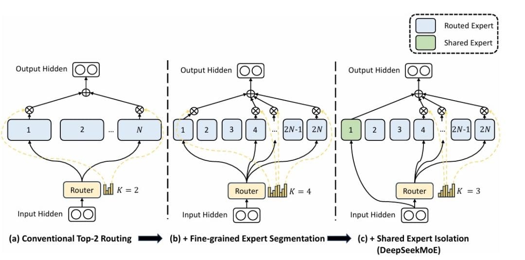
 knowledgeable networks, every with the identical structure as a regular FFN:
 = text{SwiGLU}(x)")
 . As an alternative of utilizing all consultants for each token, we choose the top-k consultants. The choice is decided by a discovered routing operate:
 = text{softmax}(x W_r + b) in mathbb{R}^N")
 is the router weight matrix and
  is a learnable bias vector. This provides us a likelihood distribution over consultants for every token.
 = {i mid r_i(x) text{ is in the top-k values of } r(x)}")
 = sum_{i in mathcal{T}_k(x)} dfrac{r_i(x)}{sum_{j in mathcal{T}_k(x)} r_j(x)} E_i(x)")
}{sum_{j in mathcal{T}_k(x)} r_j(x)}") ensures the chosen consultants’ weights sum to 1.
ensures the chosen consultants’ weights sum to 1. consultants and
  (our configuration), every token prompts 2 out of 4 consultants. If every knowledgeable has the identical measurement as a regular FFN, we’ve
  the parameters however solely
  the computation per token. That is the MoE effectivity benefit: parameter rely scales with
  .
. = text{SiLU}(text{gate}(x)) odot text{up}(x)")
 = x W_text{gate}") : tasks enter to hidden dimension
: tasks enter to hidden dimension = x W_text{up}") : is one other projection to hidden dimension
: is one other projection to hidden dimension = x cdot sigma(x)") : is the Swish activation (easy model of ReLU)
: is the Swish activation (easy model of ReLU) : denotes element-wise multiplication
)")
 activation offers easy gradients all over the place, enhancing coaching dynamics in comparison with ReLU’s laborious threshold.
 = text{SharedExpert}(x) + sum_{i in mathcal{T}_k(x)} w_i E_i(x)")
^2")
 is the variety of tokens routed to knowledgeable
  ,
,  is batch measurement, and
  is a coefficient. Nevertheless, auxiliary losses add complexity and require cautious tuning.
 denote the utilization (variety of tokens) of knowledgeable
 , is up to date as:
 ,
, is the educational charge controlling the magnitude of the bias adjustment.
") ,
, measures similarity. By minimizing this loss, we encourage sequences to be complementary — if sequence A makes use of consultants 1 and a pair of closely, sequence B ought to use consultants 3 and 4.
") that’s significantly good in some area of the enter area. The router operate
that’s significantly good in some area of the enter area. The router operate ") implicitly partitions the enter area, assigning totally different areas to totally different consultants. That is just like a combination of consultants in classical machine studying, however discovered end-to-end via backpropagation.
implicitly partitions the enter area, assigning totally different areas to totally different consultants. That is just like a combination of consultants in classical machine studying, however discovered end-to-end via backpropagation.
 is the fraction of tokens routed to knowledgeable
  is the common routing likelihood. This requires tuning
 :
:
 ),
),  ):
):

 (negligible)

 2.75M FLOPs per token
 FLOPs. Our MoE makes use of