

November 12, 2020
I lately encountered this cool paper in a studying group presentation:
It is frankly taken me a very long time to grasp what was happening, and it took me weeks to write down this half-decent rationalization of it. The first notes I wrote adopted the logic of the paper extra, this on this publish I believed I would just give attention to the excessive degree concept, after which hopefully the paper is extra simple. I needed to seize the important thing concept, with out the distractions of RNN hidden states, and so forth, which I discovered complicated to consider.
POMDP setup
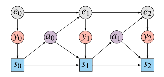
To begin with the fundamentals, this paper offers with the partially noticed Markov determination course of (POMDP) setup. The diagram under illustrates what is going on on:
The gray nodes $e_t$ present the unobserved state of the atmosphere at every timestep $t=0,1,2ldots$. At every timestep the agent observes $y_0$ which depends upon the present state of the atmosphere (red-ish nodes). The agent then updates their state $s_t$ primarily based on its previous state $s_{t-1}$, the brand new commentary $y_t$, and the earlier motion taken $a_{t-1}$. That is proven by the blue squares (they’re squares, signifying that this node relies upon deterministically on its mother and father). Then, primarily based on the agent’s state, it chooses an motion $a_t$ from by sampling from coverage $pi(a_tvert s_t)$. The motion influences how the atmosphere’s state, $e_{t+1}$ adjustments.
We assume that the agent’s final objective is to maximise reward on the final state at time $T$, which we assume is a deterministic operate of the commentary $r(y_T)$. Consider this reward because the rating in an atari sport, which is written on the display whose contents are made obtainable in $y_t$.
The final word objective
Let’s begin by stating what we in the end would love estimate from the information we have now. The belief is that we sampled the information utilizing some coverage $pi$, however we wish to have the ability to say how nicely a special coverage $tilde{pi}$ would do, in different phrases, what could be the anticipated rating at time $T$ if as a substitute of $pi$ we used a special coverage $tilde{pi}$.
What we’re inquisitive about, is a causal/counterfactual question:
$$
mathbb{E}_{tausimtilde{p}}[r(y_T)],
$$
the place $tau = [(s_t, y_t, e_t, a_t) : t=0ldots T]$ denotes a trajectory or rollout as much as time $T$, and $tilde{p}$ denotes the generative course of when utilizing coverage $tilde{pi}$, that’s:
$$
tilde{p}(tau) = p(e_0)p(y_0vert e_0) tilde{pi}(a_0vert s_0) p(s_0)prod_{t=1}^T p(e_tvert a_{t-1}, e_{t-1}) p(y_tvert e_t) tilde{pi}(a_tvert s_t) delta (s_t – g(s_{t-1}, y_t))
$$
I known as this a causal or counterfactual question, as a result of we’re inquisitive about making predictions below a special distribution $tilde{p}$ than $p$ which we have now observations from. The distinction between $tilde{p}$ and $p$ might be known as an intervention, the place we substitute particular elements within the information producing course of with totally different ones.
There are – a minimum of – two methods one might go about estimating such counterfactual distribution:
- model-free, through significance sampling. This methodology tries to immediately estimate the causal question by calculating a weighted common over the noticed information. The weights are given by the ratio between $tilde{pi}(a_tvert s_t)$, the likelihood by which $tilde{pi}$ would select an motion and $pi(a_tvert s_t)$, the likelihood it was chosen by the coverage that we used to gather the information. An incredible paper explaining how this works is (Bottou et al, 2013). Significance sampling because the benefit that we do not have to construct any mannequin of the atmosphere, we are able to immediately consider the typical reward from the samples we have now, utilizing solely $pi$ and $tilde{pi}$ to calculate the weights. The draw back, nevertheless, is that significance sampling typically extremely excessive variance estimate, and is barely dependable if $tilde{pi}$ and $pi$ are very shut.
- model-based, through causal calculus. If potential, we are able to use do-calculus to specific the causal question in an alternate approach, utilizing numerous conditional distributions estimated from the noticed information. This method has the drawback that it requires us construct a mannequin from the information first. We then use the conditional distributions discovered from the information to approximate the amount of curiosity by plugging them into the components we bought from do-calculus. If our fashions are imperfect, these imperfections/approximation errors can compound when the causal estimand is calculated, doubtlessly resulting in massive biases and inaccuracies. Alternatively, our fashions could also be correct sufficient to extrapolate to conditions the place significance weighting could be unreliable.
On this paper, we give attention to fixing the issue with causal calculus. This requires us to construct a mannequin of noticed information, which we are able to then use to make causal predictions. The important thing query this paper asks is
How a lot of the information do we have now to mannequin to have the ability to make the sorts of causal inferences we wish to make?
Choice 1: mannequin (virtually) every little thing
A technique we are able to reply the question above is to mannequin the joint distribution of every little thing, or principally every little thing, that we are able to observe. For instance, we might construct a full autoregressive mannequin of observations $y_t$ conditioned on actions $a_t$. In essence this might quantity to becoming a mannequin to $p(y_{0:T}vert a_{0:T})$.
If we had such mannequin, we might theoretically have the ability to make causal predictions, for causes I’ll clarify later. Nonetheless, this selection is dominated out within the paper as a result of we assume the observations $y_t$ are very excessive dimensional, resembling photographs rendered in a pc sport. Thus, modelling the joint distribution of the entire commentary sequence $y_{1:T}$ precisely is hopeless and would require loads of information. Due to this fact, we wish to get away with out modelling the entire commentary sequence $y_{1:T}$, which brings us to partial fashions.
Choice 2: partial fashions
Partial fashions attempt to keep away from modelling the joint distribution of high-dimensional observations $y_{1:T}$ or agent-state sequences $s_{0:T}$, and give attention to modelling immediately the distribution of $r(y_T)$ – i.e. solely the reward part of the final commentary, given the action-sequence $a_{0:T}$. That is clearly quite a bit simpler to do, as a result of $r(y_T)$ is assumed to be a low-dimensional side of the complete commentary $y_T$, so all we have now to be taught is a mannequin of a scalar conditioned on a sequence of actions $q_theta(r(y_T)vert a_{0:T})$. We all know very nicely methods to match such fashions to practical quantities of information.
Nonetheless, if we do not embrace both $y_t$ or $s_t$ in our mannequin, we can’t have the ability to make the counterfactual inferences we needed to make within the first place. Why? Let’s take a look at he information producing course of as soon as extra:
We are attempting to mannequin the causal influence of actions $a_0$ and $a_1$ on the end result $y_2$. Let’s give attention to $a_1$. $y_2$ is clearly statistically depending on $a_1$. Nonetheless, this statistical dependence emerges resulting from fully totally different results:
- causal affiliation: $a_1$ influences the state of the atmosphere $e_2$, leading to an commentary $y_2$. Due to this fact, $a_1$ has an direct causal impact on $y_2$, mediated by $e_2$
- spurious affiliation resulting from confounding: The unobserved hidden state $e_1$ is a confounder between the motion $a_1$ and the commentary $y_2$. The state $e_1$ has an oblique causal impact on $a_1$ mediated by the commentary $y_1$ and the agent’s state $s_1$. Equally $e_1$ has an oblique impact on $y_2$ mediated by $e_2$.
I illustrated these two sources of statistical affiliation by colour-coding the totally different paths within the causal graph. The blue path is the confounding path: correlation is induced as a result of each $a_1$ and $y_2$ have $e_1$ as causal ancestor. The pink path is the causal path: $a_1$ not directly influences $y_2$ through the hidden state $e_2$.
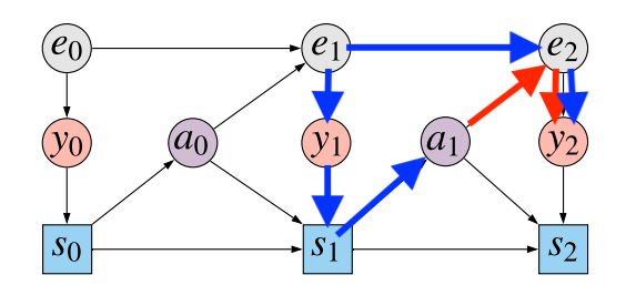
If we wish to appropriately consider the consequence of adjusting insurance policies, we have now to have the ability to disambiguate between these two sources of statistical affiliation, eliminate the blue path, and solely take the pink path into consideration. Sadly, this isn’t potential in a partial mannequin, the place we solely mannequin the distribution of $y_2$ conditional on $a_0$ and $a_1$.
If we need to draw causal inferences, we should mannequin the distribution of a minimum of one variable alongside blue path. Clearly, $y_1$ and $s_1$ are theoretically observable, and are on the confounding path. Including both of those to our mannequin would enable us to make use of the backdoor adjustment components (defined within the paper). Nonetheless, this might take us again to Choice 1, the place we have now to mannequin the joint distribution of both sequences of observations $y_{0:T}$ or sequences of states $s_{0:T}$, each assumed to be high-dimensional and tough to mannequin.
Choice 3: causally right partial fashions
So we lastly bought to the core of what’s proposed within the paper: a form of halfway-house between modeling every little thing and modeling too little. We’re going to mannequin sufficient variables to have the ability to consider causal queries, whereas preserving the dimensionality of the mannequin we have now to suit low. To do that, we modify the information producing course of barely – by splitting the coverage into two phases:
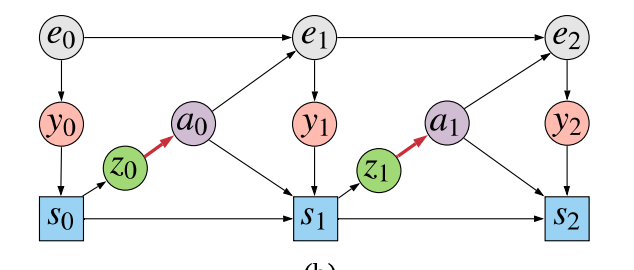
The agent first generates $z_t$ from the state $s_t$, after which makes use of the sampled $z_t$ worth to decide $a_t$. One can perceive $z_t$ as being a stochastic bottleneck between the agent’s high-dimensional state $s_t$, and the low-dimensional motion $a_t$. The belief is that the sequence $z_{0:T}$ ought to be quite a bit simpler to mannequin than both $y_{0:T}$ or $s_{0:T}$. Nonetheless, if we now construct a mannequin $p(r(y_T), z_{0:T} vert a_{0:T})$ at the moment are ready to make use of this mannequin consider the causal queries of curiosity, thanks for the backdoor adjustment components. For methods to exactly do that, please discuss with the paper.
Intuitively, this method helps by including a low-dimensional stochastic node alongside the confounding path. This enables us to compensate for confounding, with out having to construct a full generative mannequin of sequences of high-dimensional variables. It permits us to unravel the issue we have to clear up with out having to unravel a ridiculously tough subproblem.