Utilizing resampling strategies to detect influential factors

As acknowledged within the documentation for jackknife, an usually forgotten utility for this command is the detection of overly influential observations.

Some instructions, like logit or stcox, include their very own set of prediction instruments to detect influential factors. Nonetheless, these sorts of predictions could be computed for just about any regression command. Specifically, we’ll see that the dfbeta statistics could be simply computed for any command that accepts the jackknife prefix. dfbeta statistics permit us to visualise how influential some observations are in contrast with the remaining, regarding a selected parameter.

We will even compute Cook dinner’s probability displacement, which is an total measure of affect, and it can be in contrast with a selected threshold.

Utilizing jackknife to compute dfbeta

The principle process of jackknife is to suit the mannequin whereas suppressing one remark at a time, which permits us to see how a lot outcomes change when every remark is suppressed; in different phrases, it permits us to see how a lot every remark influences the outcomes. A really intuitive measure of affect is dfbeta, which is the quantity {that a} specific parameter modifications when an remark is suppressed. There might be one dfbeta variable for every parameter. If (hatbeta) is the estimate for parameter (beta) obtained from the complete information and ( hatbeta_{(i)} ) is the corresponding estimate obtained when the (i)th remark is suppressed, then the (i)th ingredient of variable dfbeta is obtained as

[dfbeta = hatbeta – hatbeta_{(i)}]

Parameters (hatbeta) are saved by the estimation instructions in matrix e(b) and likewise could be obtained utilizing the _b notation, as we’ll present beneath. The leave-one-out values (hatbeta_{(i)}) could be saved in a brand new file by utilizing the choice saving() with jackknife. With these two components, we are able to compute the dfbeta values for every variable.

Let’s see an instance with the probit command.

. sysuse auto, clear
(1978 Vehicle Knowledge)

. *protect unique dataset
. protect

. *generate a variable with the unique remark quantity
. gen obs =_n

. probit international mpg weight

Iteration 0:   log probability =  -45.03321
Iteration 1:   log probability = -27.914626
Iteration 2:   log probability = -26.858074
Iteration 3:   log probability = -26.844197
Iteration 4:   log probability = -26.844189
Iteration 5:   log probability = -26.844189

Probit regression                                 Variety of obs   =         74
                                                  LR chi2(2)      =      36.38
                                                  Prob > chi2     =     0.0000
Log probability = -26.844189                       Pseudo R2       =     0.4039

------------------------------------------------------------------------------
     international |      Coef.   Std. Err.      z    P>|z|     [95% Conf. Interval]
-------------+----------------------------------------------------------------
         mpg |  -.1039503   .0515689    -2.02   0.044    -.2050235   -.0028772
      weight |  -.0023355   .0005661    -4.13   0.000     -.003445   -.0012261
       _cons |   8.275464   2.554142     3.24   0.001     3.269437    13.28149
------------------------------------------------------------------------------

. *preserve the estimation pattern so every remark might be matched
. *with the corresponding replication
. preserve if e(pattern)
(0 observations deleted)

. *use jackknife to generate the replications, and save the values in
. *file b_replic
. jackknife, saving(b_replic, substitute):  probit international mpg weight
(operating probit on estimation pattern)

Jackknife replications (74)
----+--- 1 ---+--- 2 ---+--- 3 ---+--- 4 ---+--- 5
..................................................    50
........................

Probit regression                               Variety of obs      =        74
                                                Replications       =        74
                                                F(   2,     73)    =     10.36
                                                Prob > F           =    0.0001
Log probability = -26.844189                     Pseudo R2          =    0.4039

------------------------------------------------------------------------------
             |              Jackknife
     international |      Coef.   Std. Err.      t    P>|t|     [95% Conf. Interval]
-------------+----------------------------------------------------------------
         mpg |  -.1039503   .0831194    -1.25   0.215     -.269607    .0617063
      weight |  -.0023355   .0006619    -3.53   0.001    -.0036547   -.0010164
       _cons |   8.275464   3.506085     2.36   0.021     1.287847    15.26308
------------------------------------------------------------------------------

. *confirm that every one the replications have been profitable
. assert e(N_misreps) ==0

. merge 1:1 _n utilizing b_replic

    End result                           # of obs.
    -----------------------------------------
    not matched                             0
    matched                                74  (_merge==3)
    -----------------------------------------

. *see how values from replications are saved
. describe, fullnames

Comprises information from .../auto.dta
  obs:            74                          1978 Vehicle Knowledge
 vars:            17                          13 Apr 2013 17:45
 measurement:         4,440                          (_dta has notes)
--------------------------------------------------------------------------------
              storage   show    worth
variable title   sort    format     label      variable label
--------------------------------------------------------------------------------
make            str18   %-18s                 Make and Mannequin
worth           int     %8.0gc                Value
mpg             int     %8.0g                 Mileage (mpg)
rep78           int     %8.0g                 Restore Report 1978
headroom        float   %6.1f                 Headroom (in.)
trunk           int     %8.0g                 Trunk area (cu. ft.)
weight          int     %8.0gc                Weight (lbs.)
size          int     %8.0g                 Size (in.)
flip            int     %8.0g                 Flip Circle (ft.)
displacement    int     %8.0g                 Displacement (cu. in.)
gear_ratio      float   %6.2f                 Gear Ratio
international         byte    %8.0g      origin     Automobile sort
obs             float   %9.0g
foreign_b_mpg   float   %9.0g                 [foreign]_b[mpg]
foreign_b_weight
                float   %9.0g                 [foreign]_b[weight]
foreign_b_cons  float   %9.0g                 [foreign]_b[_cons]
_merge          byte    %23.0g     _merge
--------------------------------------------------------------------------------
Sorted by:
     Notice:  dataset has modified since final saved

. *compute the dfbeta for every covariate
. foreach var in mpg weight {
  2.  gen dfbeta_`var' = (_b[`var'] -foreign_b_`var')
  3. }

. gen dfbeta_cons = (_b[_cons] - foreign_b_cons)

. label var obs "remark quantity"
. label var dfbeta_mpg "dfbeta for mpg"
. label var dfbeta_weight "dfbeta for weight"
. label var dfbeta_cons "dfbeta for the fixed"

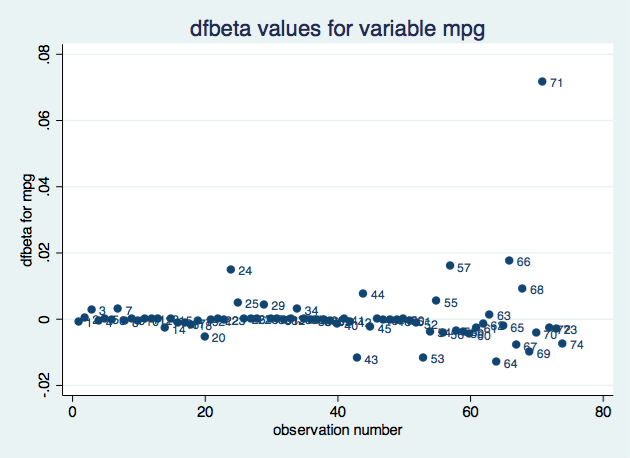
. *plot dfbeta values for variable mpg
. scatter dfbeta_mpg obs, mlabel(obs) title("dfbeta values for variable mpg")

. *restore unique dataset
. restore

Based mostly on the impression on the coefficient for variable mpg, remark 71 appears to be probably the most influential. We might create an analogous plot for every parameter.

jackknife prints a dot for every profitable replication and an ‘x’ for every replication that ends with an error. By wanting on the output instantly following the jackknife command, we are able to see that every one the replications have been profitable. Nonetheless, we added an assert line within the code to keep away from counting on visible inspection. If some replications failed, we would want to discover the explanations.

A computational shortcut to acquire the dfbeta values

The command jackknife permits us to save lots of the leave-one-out values in a special file. To make use of these, we would want to do some information administration and merge the 2 recordsdata. However, the identical command known as with the choice preserve saves pseudovalues, that are outlined as follows:

[hat{beta}_i^* = Nhatbeta – (N-1)hatbeta_{(i)} ]

the place (N) is the variety of observations concerned within the computation, returned as e(N). Due to this fact, utilizing the pseudovalues, (beta_{(i)}) values could be computed as [hatbeta_{(i)} = frac{ N hatbeta – hatbeta^*_i}{N-1} ]

Additionally, dfbeta values could be computed straight from the pseudovalues as [ hatbeta – hatbeta_{(i)} = frac{hatbeta_{i}^* -hatbeta} {N-1} ]

Utilizing the pseudovalues as an alternative of the leave-one-out values simplifies our program as a result of we don’t have to fret about matching every pseudovalue to the right remark.

Let’s reproduce the earlier instance.

. sysuse auto, clear
(1978 Vehicle Knowledge)

. jackknife, preserve: probit international  mpg weight
(operating probit on estimation pattern)

Jackknife replications (74)
----+--- 1 ---+--- 2 ---+--- 3 ---+--- 4 ---+--- 5
..................................................    50
........................

Probit regression                               Variety of obs      =        74
                                                Replications       =        74
                                                F(   2,     73)    =     10.36
                                                Prob > F           =    0.0001
Log probability = -26.844189                     Pseudo R2          =    0.4039

------------------------------------------------------------------------------
             |              Jackknife
     international |      Coef.   Std. Err.      t    P>|t|     [95% Conf. Interval]
-------------+----------------------------------------------------------------
         mpg |  -.1039503   .0831194    -1.25   0.215     -.269607    .0617063
      weight |  -.0023355   .0006619    -3.53   0.001    -.0036547   -.0010164
       _cons |   8.275464   3.506085     2.36   0.021     1.287847    15.26308
------------------------------------------------------------------------------

. *see how pseudovalues are saved
. describe, fullnames

Comprises information from /Customers/isabelcanette/Desktop/stata_mar18/309/ado/base/a/auto.
> dta
  obs:            74                          1978 Vehicle Knowledge
 vars:            15                          13 Apr 2013 17:45
 measurement:         4,070                          (_dta has notes)
--------------------------------------------------------------------------------
              storage   show    worth
variable title   sort    format     label      variable label
--------------------------------------------------------------------------------
make            str18   %-18s                 Make and Mannequin
worth           int     %8.0gc                Value
mpg             int     %8.0g                 Mileage (mpg)
rep78           int     %8.0g                 Restore Report 1978
headroom        float   %6.1f                 Headroom (in.)
trunk           int     %8.0g                 Trunk area (cu. ft.)
weight          int     %8.0gc                Weight (lbs.)
size          int     %8.0g                 Size (in.)
flip            int     %8.0g                 Flip Circle (ft.)
displacement    int     %8.0g                 Displacement (cu. in.)
gear_ratio      float   %6.2f                 Gear Ratio
international         byte    %8.0g      origin     Automobile sort
foreign_b_mpg   float   %9.0g                 pseudovalues: [foreign]_b[mpg]
foreign_b_weight
                float   %9.0g                 pseudovalues: [foreign]_b[weight]
foreign_b_cons  float   %9.0g                 pseudovalues: [foreign]_b[_cons]
--------------------------------------------------------------------------------
Sorted by:  international
     Notice:  dataset has modified since final saved

. *confirm that every one the replications have been profitable
. assert e(N_misreps)==0

. *compute the dfbeta for every covariate
. native N = e(N)

. foreach var in  mpg weight {
  2. gen dfbeta_`var' = (foreign_b_`var' - _b[`var'])/(`N'-1)
  3. }

. gen dfbeta_`cons' = (foreign_b_cons - _b[_cons])/(`N'-1)

. *plot deff values for variable weight
. gen obs = _n

. label var obs "remark quantity"

. label var dfbeta_mpg "dfbeta for mpg"

. scatter dfbeta_mpg obs, mlabel(obs) title("dfbeta values for variable mpg")

Dfbeta for grouped information

When you’ve got panel information or a scenario the place every particular person is represented by a bunch of observations (for instance, conditional logit or survival fashions), you is perhaps curious about influential teams. On this case, you’d take a look at the modifications on the parameters when every group is suppressed. Let’s see an instance with xtlogit.

. webuse towerlondon, clear
. xtset household

. jackknife, cluster(household) idcluster(newclus) preserve: xtlogit dtlm problem
. assert e(N_misreps)==0

The group-level pseudovalues might be saved on the primary observations corresponding to every group, and there might be lacking values on the remaining. To compute the dfbeta worth for the coefficient for problem, we sort

. native N = e(N_clust)
. gen dfbeta_difficulty = (dtlm_b_difficulty - _b[difficulty])/(`N'-1)

We will then plot these values:

. scatter dfbeta_difficulty newclus, mlabel(household) ///
       title("dfbeta values for variable problem") xtitle("household")

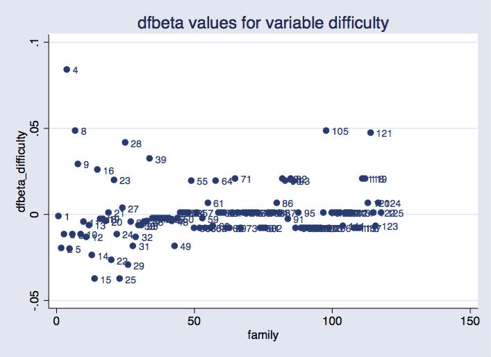
Possibility idcluster() for jackknife generates a brand new variable that assigns consecutive integers to the clusters; utilizing this variable produces a plot the place households are equally spaced on the horizontal axis.

As earlier than, we are able to see that some teams are extra influential than others. It might require some analysis to seek out out whether or not it is a downside.

Probability displacement

If we wish a world measure of affect (that’s, not tied to a specific parameter), we are able to compute the probability displacement values. We take into account the probability displacement worth as outlined by Cook dinner (1986):

[LD_i = 2[L(hattheta) – L(hattheta_{(i)})] ]

the place (L) is the log-likelihood perform (evaluated on the complete dataset), (hattheta) is the set of parameter estimates obtained from the complete dataset, and (hattheta_{(i)}) is the set of the parameter estimates obtained when leaving out the (i)th remark. Discover that what modifications is the parameter vector. The log-likelihood perform is all the time evaluated on the entire pattern; offered that (hattheta) is the set of parameters that maximizes the log probability, the log-likelihood displacement is all the time constructive. Cook dinner instructed, as a confidence area for this worth, the interval ([0, chi^2_p(alpha))), where (chi^2_p(alpha)) is the ((1-alpha)) quantile from a chi-squared distribution with (p) degrees of freedom, and (p) is the number of parameters in (theta).

To perform our assessment based on the likelihood displacement, we will need to do the following:

1. Create an (Ntimes p) matrix B, where the (i)th row contains the vector of parameter estimates obtained by leaving the (i)th observation out.
2. Create a new variable L1 such that its (i)th observation contains the log likelihood evaluated at the parameter estimates in the (i)th row of matrix B.
3. Use variable L1 to obtain the LD matrix, containing the likelihood displacement values.
4. Construct a plot for the values in LD, and add the (chi^2_p(alpha)) as a reference.

Let’s do it with our probit model.

Step 1.

We first create the macro cmdline containing the command line for the model we want to use. We fit the model and save the original log likelihood in macro ll0.

With a loop, the leave-one-out parameters are saved in consecutive rows of matrix B. It is useful to have those values in a matrix, because we will then extract each row to evaluate the log likelihood at those values.

**********Step 1
sysuse auto, clear
set more off
local cmdline probit foreign weight mpg
`cmdline'
keep if e(sample)
local ll0 = e(ll)
mat b0 = e(b)
mat b = b0

local N = _N

forvalues i = 1(1)`N'{
   `cmdline' if _n !=`i'
   mat b1 = e(b)
   mat b = b  b1
}

mat B = b[2...,1...]
mat listing B

Step 2.

In every iteration of a loop, a row from B is saved as matrix b. To guage the log probability at these values, the trick is to make use of them as preliminary values and invoke the command with 0 iterations. This may be achieved for any command that’s primarily based on ml.

**********Step 2

gen L1 = .

forvalues i = 1(1)`N'{
    mat b = B[`i',1...]
    `cmdline', from(b) iter(0)
    native ll = e(ll)
    substitute L1 = `ll' in `i'
}

Step 3.

Utilizing variable L1 and the macro with the unique log probability, we compute Cook dinner’s likehood displacement.

**********Step 3

gen LD = 2*(`ll0' - L1)

Step 4.

Create the plot, utilizing as a reference the 90% quantile for the (chi^2) distribution. (p) is the variety of columns in matrix b0 (or equivalently, the variety of columns in matrix B).

**********Step 4

native ok = colsof(b0)
gen upper_bound = invchi2tail(`ok', .1)
gen n = _n

twoway scatter LD n, mlabel(n) || line upper_bound n, ///
title("Probability displacement")

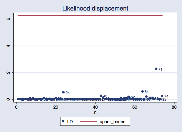
We will see that remark 71 is probably the most influential, and its probability displacement worth is inside the vary we’d usually anticipate.

Reference

Cook dinner, D. 1986. Evaluation of native affect. Journal of the Royal Statistical Society, Collection B 48: 133–169.