Understanding Phrase Embeddings (2) – Geometry

I’ve observed that after I use the time period “coordinates” to speak about vectors, it doesn’t at all times click on for everybody within the room. The earlier publish lined the algebra of phrase embeddings and now we clarify why you must take into consideration the vector of the phrase embedding merely as coordinates in house. We skip the trivial 1D and 2D circumstances since they’re simple. 4 dimensions is just too sophisticated for me to gif round with, so 3D dimensions must suffice for our illustrations.

Geometric interpretation of a phrase embedding

Check out this primary matrix:

The one-hot word-vectors are visualized within the 3D house as follows: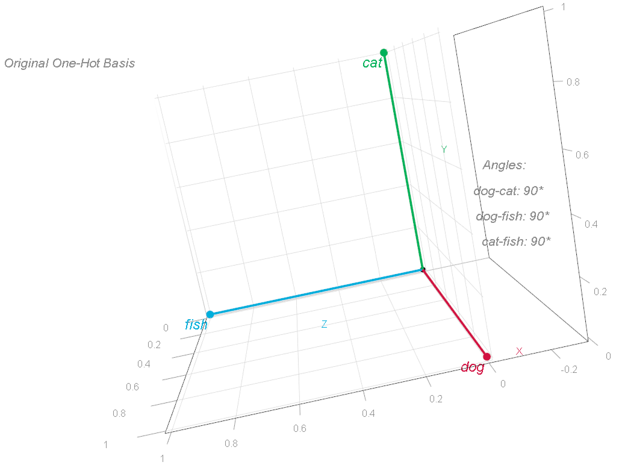

To raised perceive this coordinate system, we are able to rotate these vectors. This modifications the phrases’ coordinates, however preserves their relationships—particularly, the angles between them stays at 90°.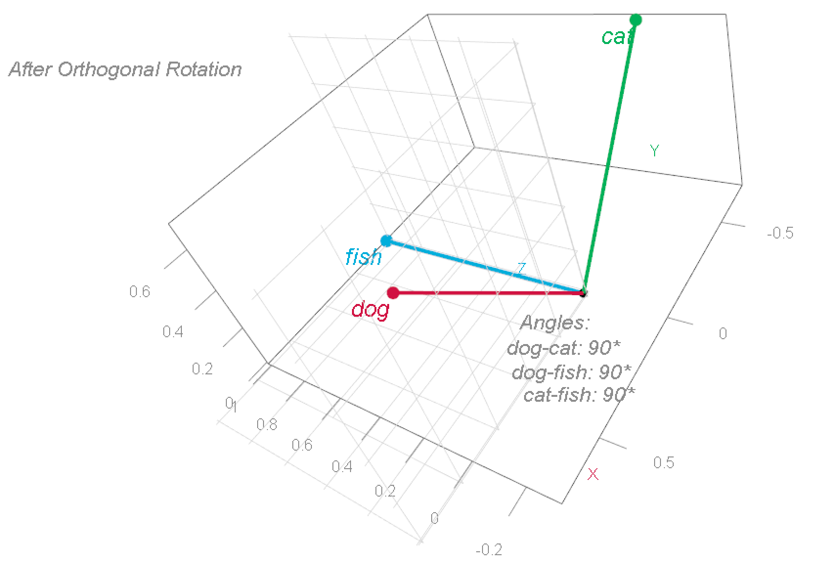

Observe that he phrase fish remained the place it was, the phrase cat now sits at [-0.707, 0.707, 0] and the phrase canine sits at [0.707, 0.707, 0], however the relationship between the phrases has not modified (it’s a 3d picture, the angles are nonetheless 90° aside). This illustrates a selected instance for what is known as “foundation transformation” (the time period “foundation” is defined within the earlier publish).

Foundation transformation in our context of phrase embeddings signifies that we alter our rudimentary one-hot illustration, the place phrases are represented in the usual foundation, to the embedding illustration the place phrases are represented in a semantic foundation.

Semantic foundation 🤨 ? Sure, let me clarify. Semantics is the department of linguistics and logic involved with that means. However, “that means” is a latent and ill-defined idea. There are other ways to explain what one means: each “inflation” and “rising-prices” map to virtually equivalent that means. Associated to that, a frequent false impression within the area of NLP matter modeling is the idea that matters are actually-defined issues, which they don’t seem to be. In reality, we would think about ourselves lucky if a subject may even not directly be inferred from the phrases assigned to the identical cluster (e.g., “matter 3”). As an illustration, if phrases like deflation, stagflation, and inflation seem collectively in the identical cluster, we may interpret that cluster as “worth stability” matter – even when, because it occurs, the cluster additionally contains many different, unrelated, phrases. So once we confer with semantics, we’re mainly speaking concerning the underlying, unobservedabstractlatent and ill-defined time period: that means.

What makes an area semantic is how phrases join to one another. That’s totally different from the instance above the place every phrase simply stands by itself – ‘cat’ doesn’t have any particular relationship to ‘canine’ or ‘fish’, all three phrases are alone standing.

Now that we perceive the time period “semantic”, let’s see what’s gained by shifting from our clear and exact one-hot encoding house, to a semantic house.

Phrase Coordinates in Semantic House

Semantic house is healthier than a proper/symbolic/non-semantic house largely because of these two benefits:

1. Dimension discount (we save storage- and computational prices).
2. We are able to relate phrases to one another. It’s useful if phrases like revenues and earnings aren’t completely impartial algebraically, as a result of in actuality they don’t seem to be impartial in what they imply for us (e.g. each phrases suggest to doubtlessly larger earnings).

Unpacking in progress:

1. Dimension discount: In a single-hot word-representation every phrase is totally distinct (all 90°, i.e. impartial). Phrases share no widespread parts and are utterly dissimilar (similarity=0) in that illustration. The upside is that we seize all phrases in our vocabulary and every phrase has a transparent particular location. However, that house is very large: every vector is of dimension equals to the variety of distinctive phrases (vocabulary). Once we embed word-vectors we solid every word-vector right into a decrease dimension house. As a substitute of a coordinate system with dimensions, we use a lower-dimension coordinate system, say 768. Now every phrase will not be the place it needs to be precisely. Why not? as a result of we don’t have entries to put that phrase in house, we solely have 768, so every phrase can be positioned someplace inside our 768 coordinate system. By compressing all these phrases into simply 768 dimensions, we produce a denser representations as an alternative of the extraordinarily sparse one-hot vectors. We inevitably lose the independence that one-hot encodings supplied, however this additionally presents a chance to compress the phrases in a method that locations associated phrases nearer collectively within the compressed 768 dimensional house.
2. We are able to relate phrases to one another: For the next dense word-vectors illustration (being silent for now about easy methods to discover these vectors)

      

   The plot beneath exhibits ‘cat’ and ‘canine’ are spatially nearer, indicating their larger semantic similarity in comparison with their similarity with ‘fish’.

   I received’t get into the small print of how we discover these dense word-vectors. The quick model is that we some transformer mannequin to create these vectors for us. The transformers household of fashions has the good energy to, properly.. remodel an preliminary and imprecise, a guess if you’ll, set of coordinates (word-vectors), into a way more cheap one. Cheap in that phrases finally find yourself positioned close to different phrases that relate to them (assume again to our ‘revenues’ and ‘earnings’ instance).

Observe that we didn’t exhibit dimension discount right here (the illustration stayed in 3 dimensions), this illustration targeted solely on the acquisition of that means.

To exemplify dimension discount we may can map the three vectors right into a 2 dimensional house: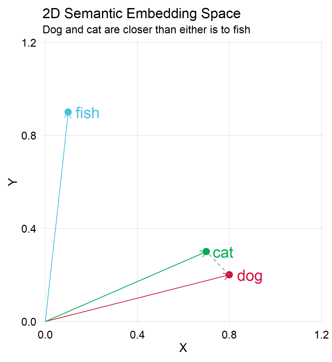

As talked about, dimension discount helps cut back storage and compute prices, however will we lose something? Completely we do.

The Crowding Drawback

Discover that within the 3d house, our one-hot foundation could be positioned such that each one vectors are perpendicular to one another. This isn’t doable in a 2nd house. However we intentionally selected a projection that maintains key distinctions, in our easy instance: maintaining “canine” and “cat” shut to one another whereas “fish” is distant. What about larger dimensions?

When decreasing dimensionality from the precise one-hot house, with the variety of vectors within the tons of of hundreds, to a smaller house, say 768 dimensions, we distort our illustration, name it compression prices. Merely put, half one million factors, as soon as dwelling massive, now should cram into an affordable dorms, with some tokens loud night breathing greater than others. This compression-induced distortion is understood by the evocative time period ‘the crowding drawback’. You might have questioned (I do know I did) why will we cease at pretty reasonable dimensions? Early language fashions had dimensions of 128, then 512, 768, 1024, 3072 and lately 4096 and that’s about it. Don’t we achieve higher accuracy if we use say ?

We don’t. Enter the Johnson-Lindenstrauss (JL) Lemma.

The Johnson-Lindenstrauss (JL) Lemma

One variation of the lemma is:
Let , and let be a set of factors. Then, for any integer , there exists a linear map such that for all :

the place is The perform that maps factors from high-dimensional house to low-dimensional house. are the projections of factors and within the lower-dimensional house. Particularly the place is the projection matrix. If you’re studying this you most likely know what PCA is, so take into consideration because the rotation matrix; to seek out the primary few elements you should multiply the unique variables with the primary few rotation-vectors. is the Euclidean norm (squared distance), and eventually is the distortion parameter (usually between 0 and 1).

Merely talking, the JL lemma states {that a} set of factors, a degree in our context is a word-vector, in high-dimensional house could be mapped into an area of dimension (a lot decrease than ..) whereas nonetheless preserving pairwise distances as much as an element of . For instance, 100,000 factors (vocabulary of 100,000) could be theoretically mapped to

Setting signifies that we settle for a distortion of 10%; so if the unique distance between vector and vector is , then after the compression it will likely be between and .

Remarks:

• Enjoyable truth: in sufficiently massive dimension even random projection – the place , with the vectors of merely drawn randomly, additionally roughly preserves pairwise distances. You may (ought to) compress massive dimensional information with out rigorously engineering , for instance you don’t at all times should spend time doing singular worth decomposition. I go away it for the curious reader to test this counter-intuitive truth.
• As typical information are, many of the construction is usually captured by the primary few dimensions. Once more, you possibly can take into consideration the primary few elements as capturing many of the variation within the information. Including elements past a sure level can add worth, however with sharply diminishing returns. One other enjoyable truth (maybe I ought to rethink my notion of enjoyable 🥴), you seize many of the variation with the primary few dimensions even when the info is totally random (that means no construction to be captured in any way). This truth was flagged lately within the prestigious Econometrica journal as spurious elements (seems to be like an element however merely the results of the numerical process).
• As oppose to the curse of dimensionality, we are able to consider the flexibility to compress high-dimensional information with out dropping a lot info because the blessing of dimensionality, as a result of it’s merely the flip facet of the curse. It cuts each methods: it’s pretty simple to shrink high-dimensional areas down as a result of factors in that house are so spread-out, which is precisely why discovering significant patterns in high-dimensional house is such a headache to start with.

In sum

We moved from one-hot illustration of phrases in a high-dimensional house to a lower-dimensional “semantic house” the place phrase relationships are captured. We confirmed how phrase vectors could be rotated with out altering their relative positions. This transformation is essential as a result of it permits us to characterize phrase that means and relationships, decreasing storage and computation prices. We then moved on to the “crowding drawback” that arises from dimensionality discount and launched the Johnson-Lindenstrauss (JL) Lemma, which supplies the theoretical legitimacy for compressing high-dimensional textual content information.

I hope you now have a greater grip on: