

Final time, I confirmed you a technique to graph and to consider matrices. This time, I need to apply the method to eigenvalues and eigenvectors. The purpose is to present you an image that may information your instinct, simply because it was beforehand.
Earlier than I’m going on, a number of individuals requested after studying half 1 for the code I used to generate the graphs. Right here it’s, each for half 1 and half 2: matrixcode.zip.
The eigenvectors and eigenvalues of matrix A are outlined to be the nonzero x and λ values that clear up
Ax = λx
I wrote quite a bit about Ax within the final put up. Simply as beforehand, x is a degree within the unique, untransformed area and Ax is its remodeled worth. λ on the right-hand aspect is a scalar.
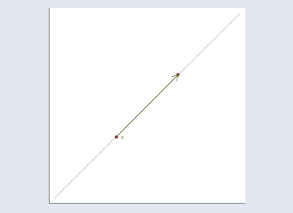
Multiplying a degree by a scalar strikes the purpose alongside a line that passes by way of the origin and the purpose:
The determine above illustrates y=λx when λ>1. If λ have been lower than 1, the purpose would transfer towards the origin and if λ have been additionally lower than 0, the purpose would go proper by the origin to land on the opposite aspect. For any level x, y=λx will likely be someplace on the road passing by way of the origin and x.
Thus Ax = λx means the remodeled worth Ax lies on a line passing by way of the origin and the unique x. Factors that meet that restriction are eigenvectors (or extra accurately, as we are going to see, eigenpoints, a time period I simply coined), and the corresponding eigenvalues are the λ‘s that report how far the factors transfer alongside the road.
Truly, if x is an answer to Ax = λx, then so is each different level on the road by way of 0 and x. That’s straightforward to see. Assume x is an answer to Ax = λx and substitute cx for x: Acx = λcx. Thus x will not be the eigenvector however is merely a degree alongside the eigenvector.
And with that prelude, we are actually able to interpret Ax = λx totally. Ax = λx finds the traces such that each level on the road, say, x, remodeled by Ax strikes to being one other level on the identical line. These traces are thus the pure axes of the rework outlined by A.
The equation Ax = λx and the directions “clear up for nonzero x and λ” are misleading. A extra trustworthy technique to current the issue could be to rework the equation to polar coordinates. We’d have stated to seek out θ and λ such that any level on the road (r, θ) is remodeled to (λr, θ). Nonetheless, Ax = λx is how the issue is often written.
Nonetheless we state the issue, right here is the image and resolution for A = (2, 1 1, 2)

I used Mata’s eigensystem() perform to acquire the eigenvectors and eigenvalues. Within the graph, the black and inexperienced traces are the eigenvectors.
The primary eigenvector is plotted in black. The “eigenvector” I bought again from Mata was (0.707 0.707), however that’s only one level on the eigenvector line, the slope of which is 0.707/0.707 = 1, so I graphed the road y = x. The eigenvalue reported by Mata was 3. Thus each level x alongside the black line strikes to 3 instances its distance from the origin when remodeled by Ax. I suppressed the origin within the determine, however you’ll be able to spot it as a result of it’s the place the black and inexperienced traces intersect.
The second eigenvector is plotted in inexperienced. The second “eigenvector” I bought again from Mata was (-0.707 0.707), so the slope of the eigenvector line is 0.707/(-0.707) = -1. I plotted the road y = –x. The eigenvalue is 1, so the factors alongside the inexperienced line don’t transfer in any respect when remodeled by Ax; y=λx and λ=1.
Right here’s one other instance, this time for the matrix A = (1.1, 2 3, 1):

The primary “eigenvector” and eigenvalue Mata reported have been… Wait! I’m getting uninterested in quoting the phrase eigenvector. I’m quoting it as a result of laptop software program and the mathematical literature name it the eigenvector although it’s only a level alongside the eigenvector. Truly, what’s being described will not be even a vector. A greater phrase could be eigenaxis. Since this posting is pedagogical, I’m going to seek advice from the computer-reported eigenvector as an eigenpoint alongside the eigenaxis. While you return to the actual world, bear in mind to make use of the phrase eigenvector.
The primary eigenpoint and eigenvalue that Mata reported have been (0.640 0.768) and λ = 3.45. Thus the slope of the eigenaxis is 0.768/0.640 = 1.2, and factors alongside that line — the inexperienced line — transfer to three.45 instances their distance from the origin.
The second eigenpoint and eigenvalue Mata reported have been (-0.625 0.781) and λ = -1.4. Thus the slope is -0.781/0.625 = -1.25, and factors alongside that line transfer to -1.4 instances their distance from the origin, which is to say they flip sides after which transfer out, too. We noticed this flipping in my earlier posting. Chances are you’ll do not forget that I put a small circle and triangle on the backside left and backside proper of the unique grid after which let the symbols be remodeled by A together with the remainder of area. We noticed an instance like this one, the place the triangle moved from the top-left of the unique area to the bottom-right of the remodeled area. The area was flipped in one among its dimensions. Eigenvalues save us from having to have a look at footage with circles and triangles; when a dimension of the area flips, the corresponding eigenvalue is adverse.
We examined close to singularity final time. Let’s look once more, and this time add the eigenaxes:

The blue blob going from bottom-left to top-right is each the compressed area and the primary eigenaxis. The second eigenaxis is proven in inexperienced.
Mata reported the primary eigenpoint as (0.789 0.614) and the second as (-0.460 0.888). Corresponding eigenvalues have been reported as 2.78 and 0.07. I ought to point out that zero eigenvalues point out singular matrices and small eigenvalues point out practically singular matrices. Truly, eigenvalues additionally replicate the size of the matrix. A matrix that compresses the area may have all of its eigenvalues be small, and that isn’t a sign of close to singularity. To detect close to singularity, one ought to take a look at the ratio of the biggest to the smallest eigenvalue, which on this case is 0.07/2.78 = 0.03.
Regardless of appearances, computer systems don’t discover 0.03 to be small and thus don’t consider this matrix as being practically singular. This matrix provides computer systems no drawback; Mata can calculate the inverse of this with out shedding even one binary digit. I point out this and present you the image in order that you should have a greater appreciation of simply how squished the area can grow to be earlier than computer systems begin complaining.
When do well-programmed computer systems complain? Say you’ve got a matrix A and make the above graph, however you make it actually massive — 3 miles by 3 miles. Lay your graph out on the bottom and hike out to the center of it. Now get down in your knees and get out your ruler. Measure the unfold of the compressed area at its widest half. Is it an inch? That’s not an issue. One inch is roughly 5*10-6 of the unique area (that’s, 1 inch by 3 miles large). If that have been an issue, customers would complain. It isn’t problematic till we get round 10-8 of the unique space. Determine about 0.002 inches.
There’s extra I might say about eigenvalues and eigenvectors. I might point out that rotation matrices haven’t any eigenvectors and eigenvalues, or at the least no actual ones. A rotation matrix rotates the area, and thus there aren’t any remodeled factors which are alongside their unique line by way of the origin. I might point out that one can rebuild the unique matrix from its eigenvectors and eigenvalues, and from that, one can generalize powers to matrix powers. It seems that A-1 has the identical eigenvectors as A; its eigenvalues are λ-1 of the unique’s. Matrix AA additionally has the identical eigenvectors as A; its eigenvalues are λ2. Ergo, Ap could be shaped by reworking the eigenvalues, and it seems that, certainly, A½ actually does, when multiplied by itself, produce A.