

My first statistics course primarily consisted of plugging numbers into formulation. I didn’t depart that course with any actual concept of how statistics differed from primary algebra. The subsequent course I took is what put all of it collectively, and I’ve cherished statistics ever since. In that course, we examined the relationships between a inhabitants and its samples. I discovered that utilizing only a small quantity of knowledge, statistics allows us to make inferences about all the inhabitants. Now that’s cool!
On this weblog, I present instruments for introductory statistics course instructors to show the ideas of sampling distributions, normal errors, confidence intervals (CIs), and p-values. For example these ideas, we’ll use the next analysis query:
Do residents of Faculty Station, TX (CSTX), who’ve been identified with diabetes have a better common physique mass index (BMI) than CSTX residents and not using a diabetes prognosis?
The inhabitants
You probably have a dataset to make use of as a inhabitants—great! Use that. Or you’ll be able to have your college students accumulate knowledge, for instance, from each eleventh grader. In any other case, you’ll have to simulate a inhabitants dataset. I’ve no means to gather knowledge from everybody in CSTX, so I’ll show utilizing a simulated inhabitants.
First, I create a brand new knowledge body referred to as inhabitants and alter into it.
. body create inhabitants
. body change inhabitants
I set a random-number seed to make sure reproducibility and set the variety of observations. I’m utilizing 135,000 as a result of that’s the estimated variety of residents in CSTX, my inhabitants.
. set seed 12
. set obs 135000
Variety of observations (_N) was 0, now 135,000.
Then we’ll use Stata’s random-number mills to simulate BMI and diabetes incidence within the inhabitants. See [FN] Random-number capabilities, or sort assist random quantity capabilities into Stata’s Command window for a full checklist of obtainable distributions.
We’ll use a traditional distribution for BMI and a binomial distribution for diabetes. I do a fast web search to get hyperparameters for these distributions, that’s, the imply and normal deviation of BMI within the US inhabitants and the proportion with a diabetes prognosis. The variety of occasions within the binomial distribution is 1 as a result of we’re simulating just one occasion: diabetes. I add 2 to everybody within the diabetes group in order that their common BMI is 2 larger than the nondiabetic group.
. generate diabetes = rbinomial(1,0.12)
. generate bmi = rnormal(27,6) + 2 * diabetes
It’s good observe to assign labels and worth labels (if relevant) to generated variables. Let’s do
that now.
. label variable bmi "Physique mass index"
. label variable diabetes "Diabetes prognosis"
. label outline diab 0 "Not diabetic" 1 "Diabetic"
. label values diabetes diab
Samples
We are able to extract a single pattern from this inhabitants utilizing the pattern command. We’ll pattern simply 0.1% of the inhabitants. We first use protect to protect our inhabitants.
. protect
. pattern 0.1
(134,865 observations deleted)
Let’s conduct a t check on this pattern to check whether or not the imply BMI differs by diabetes group.
. ttest bmi, by(diabetes)

Two-sample t check with equal variances
------------------------------------------------------------------------------
   Group |     Obs        Imply    Std. err.   Std. dev.   [95% conf. interval]
---------+--------------------------------------------------------------------
Not diab |     114    28.31035    .5315609    5.675517    27.25723    29.36347
Diabetic |      21    29.49885      .91868    4.209921    27.58252    31.41518
---------+--------------------------------------------------------------------
Mixed |     135    28.49523    .4713703    5.476828    27.56294    29.42752
---------+--------------------------------------------------------------------
    diff |           -1.188497    1.301377                -3.76257    1.385575
------------------------------------------------------------------------------
    diff = imply(Not diab) - imply(Diabetic)                        t =  -0.9133
H0: diff = 0                                     Levels of freedom =      133

    Ha: diff < 0                 Ha: diff != 0                 Ha: diff > 0
 Pr(T < t) = 0.1814         Pr(|T| > |t|) = 0.3628          Pr(T > t) = 0.8186
The primary two sections give some details about every group and their mixed pattern. The final row, labeled diff, is what we’re testing. The distinction in means in BMI on this pattern is 1.19 (SE = 1.30; 95% CI [-3.76, 1.39]). The distinction in means estimate within the outcomes desk is damaging as a result of it subtracts the diabetic imply BMI from the nondiabetic imply BMI.
The t statistic is simply the distinction in means divided by its normal error. We are able to calculate this manually by utilizing the distinction in means and normal error within the returned outcomes.
. return checklist

scalars:
            r(ub_diff) =  1.385575269027033
            r(lb_diff) =  -3.762570056926808
            r(mu_diff) =  -1.188497393949888
        r(ub_combined) =  29.42751874623384
        r(lb_combined) =  27.56294203811313
        r(se_combined) =  .4713703167472302
        r(mu_combined) =  28.49523039217349
         r(N_combined) =  135
               r(ub_2) =  31.41518328412929
               r(lb_2) =  27.58251754333305
               r(se_2) =  .9186799859364339
               r(ub_1) =  29.36347104716379
               r(lb_1) =  27.25723499239878
               r(se_1) =  .5315609062940896
              r(degree) =  95
                 r(sd) =  5.476828159975613
               r(sd_2) =  4.209920574994674
               r(sd_1) =  5.675517392222678
                 r(se) =  1.301376679922003
                r(p_u) =  .8186212430198624
                r(p_l) =  .1813787569801376
                  r(p) =  .3627575139602752
                  r(t) =  -.9132616346107564
               r(df_t) =  133
               r(mu_2) =  29.49885041373117
                r(N_2) =  21
               r(mu_1) =  28.31035301978128
                r(N_1) =  114
We use the distinction in means, saved as r(mu_diff), and the usual error, saved as r(se), to calculate t.
. show r(mu_diff)/r(se)
-.91326163
This is similar t statistic reported below the outcomes desk. In the event you’re ever uncertain how a statistic is being calculated, go to the Strategies and formulation in [R] ttest. Utilizing this pattern, we don’t have sufficient proof to conclude that there’s a distinction between teams, t(133) = 0.91, p = 0.181. We use the lower-tail p-value as a result of our speculation is that the diabetic group had a better imply BMI than the nondiabetic group.
What if we had sampled a special set of observations? First, let’s restore after which protect our inhabitants once more.
. restore
. protect
Now, let’s use a special random-number seed, then pattern and check once more.
. set seed 78

. pattern 0.1
(134,865 observations deleted)

. ttest bmi, by(diabetes)

Two-sample t check with equal variances
------------------------------------------------------------------------------
   Group |     Obs        Imply    Std. err.   Std. dev.   [95% conf. interval]
---------+--------------------------------------------------------------------
Not diab |     119    27.38515    .5024667    5.481265    26.39013    28.38017
Diabetic |      16    30.22711    1.023486    4.093946     28.0456    32.40862
---------+--------------------------------------------------------------------
Mixed |     135    27.72197    .4649424    5.402142     26.8024    28.64155
---------+--------------------------------------------------------------------
    diff |           -2.841961    1.422678               -5.655963   -.0279588
------------------------------------------------------------------------------
    diff = imply(Not diab) - imply(Diabetic)                        t =  -1.9976
H0: diff = 0                                     Levels of freedom =      133

    Ha: diff < 0                 Ha: diff != 0                 Ha: diff > 0
 Pr(T < t) = 0.0239         Pr(|T| > |t|) = 0.0478          Pr(T > t) = 0.9761
Utilizing this pattern, we have now proof that there’s a group distinction in imply BMI, t(133) = 2.00, p = 0.024.
Let’s put this pattern right into a body referred to as pattern, then restore our inhabitants.
. body put *, into(pattern)
. restore
Pattern-to-sample variability is vital to with the ability to make statistical inferences. As a result of we have now the inhabitants, we are able to construct a sampling distribution to see this variability firsthand.
The sampling distribution
We begin by creating a brand new knowledge body named sampling with variables diff, se, ub, and lb.
. body create sampling diff se ub lb
Then we use a for loop to gather 100 samples, every containing 0.1% of the inhabitants. We conduct t assessments on every of those samples and publish the estimated distinction in means, normal error, and higher and decrease bounds of the CI to the sampling body. We add quietly in entrance of pattern and ttest to suppress their outputs.
. forvalues i = 1/100 {
  2. protect
  3. quietly pattern 0.1
  4. quietly ttest bmi, by(diabetes)
  5. body publish sampling (r(mu_diff)) (r(se)) (r(ub_diff)) (r(lb_diff))
  6. restore
  7. }
We alter to the sampling body we simply created.
. body change sampling
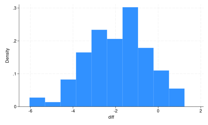
Let’s start by a histogram of the distinction in means.
. histogram diff
(bin=10, begin=-6.039753, width=.72761365)
This can be a sampling distribution of the distinction in means in BMI by diabetes prognosis. We are able to see that almost all of our samples are round -2, as anticipated, however there’s a substantial unfold. Additionally word that it’s roughly usually distributed. That is as a result of central restrict theorem, which states that the distribution of pattern technique of impartial, identically distributed random variables approaches a traditional distribution because the pattern dimension will increase, whatever the authentic inhabitants’s distribution. (Having college students begin with different inhabitants distributions is usually a enjoyable train!)
Normal error
The usual deviation of the sampling distribution is named the usual error. After we conduct a t check on a pattern, we additionally get an estimate of the usual error. It tells us in regards to the anticipated distance between our pattern estimate and the inhabitants parameter.
. summarize se diff

    Variable |        Obs        Imply    Std. dev.       Min        Max
-------------+---------------------------------------------------------
          se |        100    1.610917    .2193768   1.206266   2.400811
        diff |        100   -1.956383    1.477907  -6.039753   1.236384
The estimated normal error in response to this sampling distribution is 1.48. We see that the common estimated normal error from the samples, 1.61, is near this quantity, even with solely 100 samples. Because the variety of samples in our sampling distribution will increase, these two numbers will converge, and the distinction in means will method -2.
It’s also possible to have your college students use completely different pattern sizes when constructing a sampling distribution to see how this impacts the usual error. Use the depend possibility of the pattern command to instantly pattern a selected variety of observations slightly than a share.
CI
The CI is one other mind-set in regards to the variability throughout samples. If we repeat the sampling course of many instances, 95% of the 95% CIs constructed will comprise the true, unknown inhabitants parameter. As a result of we have now 100 samples in our sampling distribution, we anticipate 95 of them to comprise -2, the true distinction.
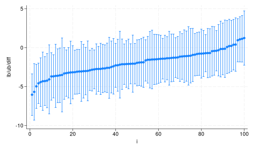
Let’s have a look at the CIs we collected from every of the samples in our sampling distribution.
We kind, then create variable i to get them organized on the x axis from smallest to largest level estimate, after which use twoway rpcap to visualise them.
. kind diff
. generate i = _n
. twoway (rpcap lb ub diff i)
Let’s add a reference line on the true distinction, -2, and add titles.
. twoway (rpcap lb ub diff i), ytitle("Distinction in means") yline(-2)
> xtitle("") xlabel(none, nolabels) title("100 95% confidence intervals")
> subtitle("95 comprise the true inhabitants parameter (dashed line)")
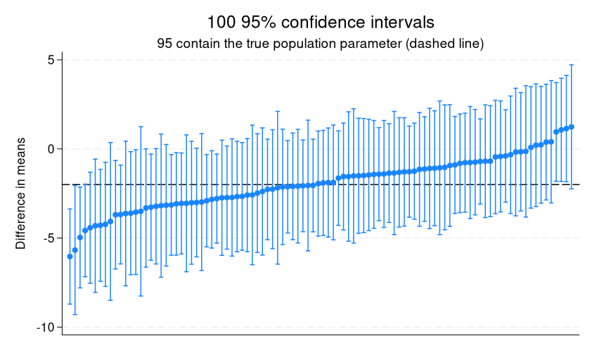
We are able to see that the primary CI and the final 4 CIs don’t comprise the true worth.
After we calculate a CI in a pattern, it’s the estimated vary of values inside which we’re 95% assured the true inhabitants parameter lies. With this demonstration, we are able to simply see that “95% assured” refers back to the share of intervals containing the true parameter throughout repeated samples slightly than the usually incorrectly used interpretation that there’s a 95% likelihood (or 0.95 chance) that the true parameter lies throughout the interval constructed from a single pattern.
p-values
There may be yet another idea I want to cowl: p-values. They’re infamously misunderstood and misused. Thus, I believe it’s vital that college students perceive what they’re and what they actually inform us.
To know p-values would require constructing a null sampling distribution, that’s, a sampling distribution from a inhabitants during which there isn’t a impact. To create a null sampling distribution, we are able to observe the identical course of we used for the choice sampling distribution with out including 2 to the diabetes group, however we don’t need to. We all know precisely what the distribution of t statistics will seem like from a null inhabitants; they are going to be t distributed! That’s why we trouble with creating check statistics within the first place.
Let’s first visualize a t distribution utilizing a twoway perform graph.
. twoway (perform density = tden(133,x), vary(-3 3)), xtitle({it:t})
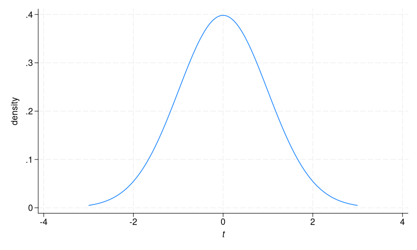
That is the sampling distribution of t values we might anticipate from a inhabitants during which there isn’t a distinction in imply BMI between diabetics and nondiabetics. As anticipated, it facilities round 0.
Let’s see the t check on our final pattern as soon as extra.
. body pattern: ttest bmi, by(diabetes)

Two-sample t check with equal variances
------------------------------------------------------------------------------
   Group |     Obs        Imply    Std. err.   Std. dev.   [95% conf. interval]
---------+--------------------------------------------------------------------
Not diab |     119    27.38515    .5024667    5.481265    26.39013    28.38017
Diabetic |      16    30.22711    1.023486    4.093946     28.0456    32.40862
---------+--------------------------------------------------------------------
Mixed |     135    27.72197    .4649424    5.402142     26.8024    28.64155
---------+--------------------------------------------------------------------
    diff |           -2.841961    1.422678               -5.655963   -.0279588
------------------------------------------------------------------------------
    diff = imply(Not diab) - imply(Diabetic)                        t =  -1.9976
H0: diff = 0                                     Levels of freedom =      133

    Ha: diff < 0                 Ha: diff != 0                 Ha: diff > 0
 Pr(T < t) = 0.0239         Pr(|T| > |t|) = 0.0478          Pr(T > t) = 0.9761
We get a t statistic of -1.99, and on the backside we see three p-values: lower-, two-, and upper-tailed.
The lower-tailed p-value tells us that if there have been no distinction in means in BMI within the inhabitants, the chance of calculating a t statistic that’s lower than -1.99 is 0.024, or about 2%. We are able to replicate this quantity utilizing the cumulative Scholar’s t distribution perform, t(df, t), the place df is the levels of freedom from our pattern, 133, and t is the t statistic from our pattern, -1.9976.
. show t(133,- 1.9976)
.02390008
This perform calculates the cumulative chance of the t distribution as much as -1.9976. To visualise this, we add an x line to our t distribution graph.
. twoway (perform density = tden(133,x), vary(-3 3)),
> xtitle({it:t}) xline(-2)
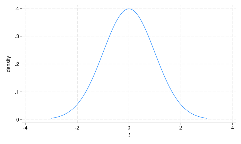
2.4% of the distribution is to the left of the dashed line.
The upper-tailed p-value tells us that if there have been no distinction in means in BMI within the inhabitants, the chance of calculating a t statistic higher than -1.99 is 0.976, or about 98%. Once more, we are able to replicate this quantity utilizing the cumulative distribution perform, this time subtracting from 1.
. show 1 - t(133,- 1.9976)
.97609992
Now we’re calculating the chance to the precise of the dashed line in our graph, which is 1 – the chance to the left.
The 2-tailed p-value is just twice the lower-valued p-value, on this case the lower-tailed.
. show 2 * t(133,- 1.9976)
.04780016
It tells us the chance of calculating a t statistic lower than -1.99 or higher than 1.99. We are able to add a second line to our graph to visualise this.
. twoway (perform density = tden(133,x), vary(-3 3)), xtitle({it:t})
> xline(-2) xline(2)
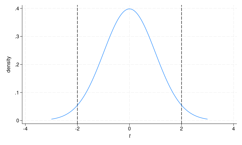
The 2-tailed p-value is the proportion to the left of the primary dashed line plus the proportion to the precise of the second dashed line. In different phrases, it’s telling us that, if there isn’t a true distinction between teams, there may be 5% chance of getting a t statistic as or extra excessive than the statistic we calculated on this pattern.
Conclusion
On this weblog, we have now explored easy methods to show the next core pillars of statistical inference by means of simulation and visualization: sampling distributions, normal errors, CIs, and p-values.
Statistics turns into compelling for college kids once they can see the relationships between a inhabitants and its samples for themselves. To convey these demonstrations into your classroom and assist your college students study a lot quicker, you’ll be able to obtain the do-file right here.