

The continual-treatment DiD paper I’ve been working by for a sequence of posts has been primarily targeted, not on the causal parameters and never on the estimators, however slightly on two-way mounted results (TWFE) and Frisch-Waugh-Lovell (FWL). I’ve been narrowly within the decomposition weights of TWFE that Callaway, Goodman-Bacon and Sant’Anna (CBS) current in Desk 1 of the paper. I’ve been presenting the “Ranges” weights in an R shiny paper hosted on my web site too. In the present day I wished to offer an outline of what precisely on this desk, and why are there 4 completely different rows within the “Decomposition” column if there is just one TWFE regression to decompose utilizing FWL?
The central truth, which I would like readers to carry mounted earlier than we go wherever else: Desk 1 is presenting decomposition weights from just one regression. Right here’s what I imply. Let’s say that you simply regress your consequence on the continual therapy dose, in a panel of two durations, with business and time mounted results. What occurs?
You get a single OLS estimate.
There’ll solely be one coefficient. We conventionally name it β-hat. And utilizing FWL, we are able to decompose it algebraically right into a set of weights consisting of a density perform (f_D(l)), deviations from the imply (l-E[D]) and variance (Var(D)). These three issues are the constructing blocks of the “Ranges” row. You may have these three, you possibly can all the time calculate the β-hat from TWFE with out ever technically operating the regression as a result of FWL allows you to calculate algebraically the regression coefficient with out really operating the regression.
However there are three different rows. So what’s going on right here? How can there be 4 rows of weights they usually all be from FWL? Would these weighted values give the identical quantity, then, if there is just one regression? What are the completely different rows doing?
Once more, let me be clear and say what they’re not doing. The 4 rows of Desk 1 are not similar to 4 completely different regressions. They’re not even 4 completely different abstract statistics you compute on the facet. Relatively, they’re 4 algebraic rewrites of the identical β-hat the place every expression of that single quantity as a weighted common of some underlying causal parameter which I’ve been avoiding for the second. OLS equals all the decomposition. One other strategy to say that’s to say that the decomposition just isn’t distinctive.
Each row of Desk 1 lands on the identical worth. What differs between rows is what that worth is a weighted common of.
Let’s be concrete and discuss once more concerning the Lu and Yu (2015) AEJ:Utilized article. Recall that China joined the WTO in 2001. This pressured any business with a pre-WTO tariff above roughly 10% to chop right down to a WTO-compliant ceiling. Industries already at or beneath the ceiling did not lower in any respect. The dimension of every business’s mandated lower was mechanically tied to how excessive its pre-WTO tariff had been. And that is the regression we’ve got been utilizing.
(y_{it} ;=; alpha_i ;+; beta^{textual content{twfe}} cdot textual content{Tariff}_{i,,2001} cdot textual content{Post02}_t ;+; lambda_t ;+; varepsilon_{it})
When a practitioner runs a regression of business outcomes on 2001 Chinese language tariffs (above) and will get a quantity (β-hat) from that OLS, they may often describe it in a single of some methods. Let me state examples of every of them.
-
“That is the impact of this system.”
-
“That is the impact of a marginal one level change within the dose.”
-
“That is the common impact of 1 unit of the dose.”
One regression — β-hat — however three distinct questions. Not completely different shades of each other. Relatively, three distinct questions. So let me elaborate on every of them.
For an business that confronted a 15 proportion level tariff in 2001, what’s the impact of that tariff on their consequence, in comparison with an business that confronted no tariff in any respect? This can be a degree impact. That is the one I’ve been working with the previous couple of substacks. That is the one which yow will discover underneath the first tab of my shiny. It’s a distinction between handled at dose l and untreated. Desk 1’s second row labeled the “ranges decomposition,” rewrites β-hat as a weighted common over degree results of this type.
However now let’s change the query away from “the impact”. Let’s take a look at a specific state of affairs and ask a unique query.
For an business already sitting at a 15-point tariff, what would occur in the event you nudged their tariff up by a tiny little sliver? What occurs?
That’s a by-product. It’s a native slope of the response curve at dose l. And as soon as we get into the causal parameters, we will map that query to a specific causal response which CBS name the ACRT. And that’s the third row of Desk 1 labeled “Scaled Ranges”. It’s β-hat rewritten as a weighted common of native slopes.
If industries with increased tariffs skilled larger consequence adjustments, you possibly can divide every business’s degree impact by its dose to get an impact per proportion level, then common. That’s the scaled degree impact. Row two.
The fourth query is slightly completely different. What if we had been to select an business with a decrease tariff l and an business with a better tariff h? after which had been to ask concerning the slope of outcomes between them per unit of tariff hole? What’s that query precisely?
Effectively, in that situation, you by no means undergo the untreated in any respect. Do you see that? In that state of affairs, you’re evaluating the excessive and low dose industries to at least one one other, to not some counterfactual the place neither is handled. You’re evaluating dose to dose. The scaled 2×2 decomposition, row 4, rewrites β-hat as a weighted common of those pairwise slopes.
So there are 4 questions in Desk 1, however there is just one regression in Desk 1.
When you maintain that β-hat mounted, you possibly can see the 4 rows in Desk 1 as 4 questions. And while you do, then you possibly can monitor the rhetoric of their paper because it strikes from merely FWL’s single interpretation to being one thing extra nuanced and a bit sharper. And right here it’s:
Does TWFE have a very good interpretation in any of them?
See, this is without doubt one of the cores of the paper. Can I take any of these 4 questions — all superb questions — and ask if my TWFE coefficient has a satisfying reply to them? The weighted averages are the reply to 4 completely different questions and the reply?
No. More often than not, no.
More often than not, β-hat from OLS is expressible as a weighted common underneath all 4 framings. And that’s purely mechanical. Purely algebraic. Pops out of FWL.
However in not one of the 4 circumstances, as we’ll see as soon as we transfer by Desk 1, which is solely about TWFE’s estimate, not one of the 4 circumstances incorporates a β-hat expression that cleanly equals the parameter that you’d have written down at the beginning of your analysis undertaking.
We begin with the estimand. The estimand is a inhabitants parameter, often a causal inhabitants parameter, and we estimate it in OLS. However, whereas the very best linear predictor (BLP) is a inhabitants abstract of the conditional expectation perform (CEF), and OLS is its implementation within the pattern, not all inhabitants estimands are the identical, and never all of them map, subsequently, onto an OLS primarily based reply. Not one of the 4 circumstances in Desk cleanly equal the causal goal parameter that you’d have doubtless written down at the beginning of your analysis undertaking. Not one of the rows in Desk 1 correspond to the inhabitants estimand which is nothing greater than an explicitly acknowledged query that may be interpreted as a causal response. So what are they?
Effectively, within the degree decomposition, the weights must sum to zero. They should. Why? As a result of take a look at the primary time period — we recentered every unit’s tariff relative to the imply. And in the event you recenter, that essentially means a number of the degree results will get destructive weights. Which of them? Effectively, the beneath common industries will get destructive weights as a result of that’s what recentering means in that case.
See beneath the pink line within the left graph’s place relation relative to the dashed line which is the imply dose in our information. Then take a look at that dose’s location on the precise graph which lands within the pink-ish zone. Then go left to the y-axis — destructive weight.
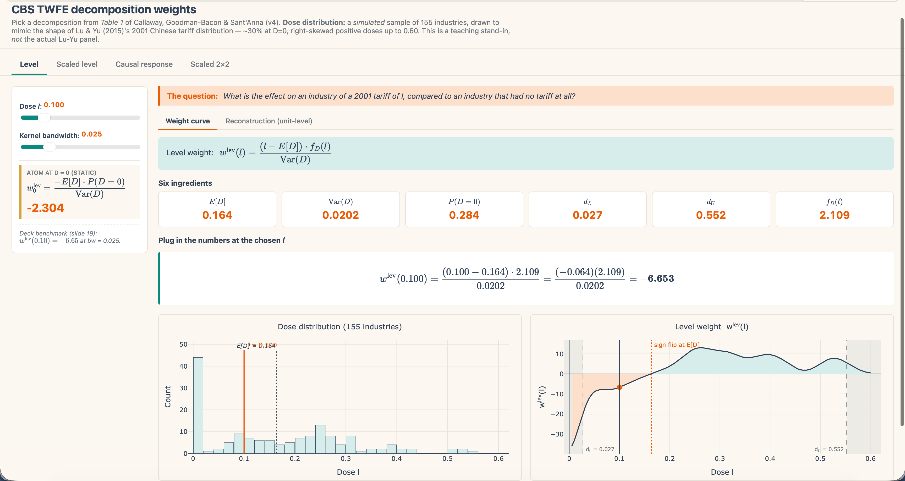
That’s the reasoning you get from recentering the dose round its imply. An business with a below-average tariff will pull β-hat down when its degree impact should be pulling β-hat up.
I’ve not but gotten into the opposite three, as I believed it was extra vital we actually nail the degrees as we’ve got to begin someplace, and I discovered that one to be the simplest to begin with.
However, right here let me give a fast heads-up to one of many others. The decomposition of β-hat rewritten because the causal response decomposition has all non-negative weights which is nicer, however weirdly they don’t correspond to the density of tariffs in your pattern. With that one, the industries with reasonable tariffs will get weighted extra closely than industries on the extremes for causes that don’t have anything to do together with your analysis design.
After which the opposite two rows are completely different variations of the identical story. These solutions to their questions will change the form, and introduce a mismatch between β-hat and any inhabitants estimand parameter of curiosity.
And bear in mind — we begin with estimands. We don’t begin with OLS. Regressions within the pattern are a part of the sampling distribution of OLS which on common underneath the regulation of enormous numbers will equal the very best linear prediction (BLP) that you possibly can run within the inhabitants, however that doesn’t imply that the BLP itself is the purpose. The purpose is all the time to reply a query the place the reply corresponds to a goal parameter, often a causal parameter.
One of many paper’s actual contributions is that the reply you need lives upstream from a regression, and OLS can not itself infer which one you requested, and can’t itself give a satisfying reply both except you set restrictions on it. So Desk 1 isnot a menu of decompositions. It’s extra like a analysis as a result of it exhibits, by the window of FWL, the interpretation of the regression coefficient from OLS.
If you want to jot down a regression coefficient as a weighted common of fine comparisons, then you’ll get destructive weights. And in the event you discover that dissatisfying and as an alternative write the regression coefficient when it comes to forbidden comparisons, you’ll get rid of the destructive weights however then must take care of the truth that you at the moment are evaluating two handled teams to at least one one other.
So let’s ask the apparent. What precisely does “good” imply in our case?
“Good” means comparisons to the untreated. Which I believe is without doubt one of the core classes a number of us realized from the sooner diff-in-diff literature, a number of which we owe to the Bacon decomposition from Andrew’s 2001 Journal of Econometrics.
comparability is about evaluating an business that confronted a tariff versus an business that confronted none. It corresponds to a specific causal parameter I’ve not but labored out, however for now simply word that such a comparability is usually known as clear, and it’s most likely intuitive in lots of contexts. It’s the Y(1)-Y(0) unit degree therapy impact summarized and averaged. It’s the core of the potential outcomes framework which expresses therapy results as comparisons to an untreated, Y(0), therapy state. That’s what the extent decomposition offers you.
However the weights in that decomposition are pressured to sum to zero by the mechanics of OLS, which we are able to solely see if we crack it open utilizing FWL like an atom smasher. And if the weights sum to zero, then they must be destructive someplace and optimistic some place else. And FWL exhibits that these destructive weights are on the industries with beneath common tariffs which you’ll see by transferring the slider round in my shiny app.
However the scaled 2×2 decomposition manages to flee the destructive weights. Each weight within the scaled 2×2 row is optimistic and sum to at least one. That is typically what folks imply after they say that averaging is “properly behaved”. They imply that the weights sum to at least one and non are destructive.
Take into consideration artificial management — the weights are non-negative and sum to at least one, which forces the artificial management to reside with out extrapolation, however on the similar time, can pressure the artificial management to utterly miss too.
Effectively you possibly can by no means measure the therapy results in actual life since you are all the time lacking one of many vital potential outcomes per unit. So all you possibly can ever do is make comparisons, and hopefully principled ones that correspond to an interpretable inhabitants estimand, or “goal parameter”. And within the scaled 2×2 from OLS, the comparisons you’re now averaging over are pairs of handled industries, with one of many pairs drawn from a decrease tariff and the opposite drawn from a better tariff.
Bacon’s 2021 Journal of Econometrics paper famously flagged comparisons like these and we now check with them because the “late versus early” comparability within the staggered binary case. They’re the “forbidden comparability” in keeping with the language we discover in different writers like Borusyak, Caravel and Speiss I believe, in addition to de Chaisemartin and D’Haultfoueille. Such comparisons introduce contamination (see Solar and Abraham 2021 too) as a result of one handled unit’s impact can infect the comparability underneath basic circumstances associated to what these therapy results are.
Effectively, within the steady world, the identical concern comes again: you’re contrasting two items which can be each within the therapy, simply in numerous quantities. And as I stated, that introduces its personal points.
And thus we see the bind that our OLS mannequin above places us in. Because the economist likes to say, there isn’t a free lunch. You’re damned in the event you do; damned in the event you don’t. But paradoxically, it’s not within the intuitive path as a result of with steady therapy, good comparability give us destructive weights by the re-centering that OLS does. And with forbidden comparisons, we get optimistic weights. And each of those are actual rewrites of the identical quantity.
I don’t need to put phrases into the authors’ mouth, however it’s virtually like Desk 1 is displaying us that all of those are forbidden comparisons apart from comparisons to untreated items. Unfavourable weights aren’t a flaw in OLS. Relatively, they’re the value of asking a clear query. In order for you each comparability in your weighted common to be an untreated-versus-treated distinction, then your weights could have indicators you don’t like. And in the event you don’t like these indicators, you must quit the cleanness. And the rows in Desk 1 are nearly choosing your poison.
So after I run OLS of business outcomes on 2001 tariff, and I get a coefficient, what query am I answering?
If I used to be asking “what’s the impact of the tariff?” within the degree sense, it’s the common distinction between an business taxed at l and an business taxed at zero. And that’s the one for the previous couple of substacks I’ve been targeted on answering. And that’s the one with destructive weights. In our simulation, the below-average-tariff industries are pulling the coefficient within the improper path.
Effectively what if I requested the marginal-effect query? If I ask the marginal-effect query, then I’m additionally getting a solution, and the weights look nicer since they gained’t be destructive as I’ll work by in a later submit, however you’ll get a weighting scheme that doesn’t match the distribution of tariffs I even have.
And if I used to be asking the per-unit query, which is a pairwise-slope query, it’s the similar story. That reply will get me a single quantity with weights which can be decided by the variance of the dose, not by something about my analysis query.
If you happen to hear shut, you possibly can really hear echoes of the Bacon decomposition of OLS with panel unit and time mounted results from the binary case with staggered diff-in-diff.
A part of the purpose of their paper is to say that not one of the 4 rewrites are the clear factor we’re often after. And nothing within the regression output tells me which of the 4 I used to be attempting to ask.
The constructive half of the CBS paper in part 4 is about what to do after we’ve got all collectively internalized all that. We have interaction in “inhabitants first” fashion reasoning, not “regression first” fashion reasoning. That’s, we resolve, up entrance, which parameter we really care about. And as soon as we’re clear about that, solely then will we construct an estimator focused at that estimand, or which these days we frequently name the goal parameter. And that’s the place we make assumptions — not calculations, however assumptions. That’s the place we separate “identification” from estimation.
We goal a clearly outlined parameter underneath clearly expressible assumptions which Pedro is keen on calling the “forward-engineered” estimator.
And it’s not simply Pedro; you possibly can see it in Mogstadt and Torgovitsky’s handbook chapter on labor economics (right here is the NBER of that) which opinions instrumental variables with “unbounded heterogenous therapy results”, which has been a recurring theme within the new diff-in-diff literature and which carries over to this paper, not surprisingly, as properly.
In order for you the common degree impact among the many handled, we are going to see as I progress that there’s a binarized DiD that delivers precisely that to us. And in order for you as an alternative the native slope at every dose, there CBS will give us what are known as “sieve” estimators that hit that immediately.
Clearly outlined, population-level, estimands with identification assumptions supporting estimators designed to offer it to us.
I’ll work by these later, although, in a future submit. The reframe I wished to do now was merely to notice that the 4 rows of Desk 1 usually are not 4 solutions. They don’t seem to be 4 solutions. Relatively, the are 4 makes an attempt to interpret the only quantity OLS gave us with one per candidate query you might need been asking. The decomposition isn’t the estimator. It’s extra just like the analysis that helps us higher perceive what OLS gave us.