

Widespread sense says that what you imagine after seeing new information needs to be some type of compromise between what you believed earlier than and what the brand new information says. You don’t need to ignore earlier data or new data.
How a lot ought to new information change your prior beliefs? When prior judgment and new data are in battle, which one needs to be given the advantage of the doubt?
Bayesian information fashions present a framework for making such choices quantitative and goal. The selection of an information mannequin is considerably subjective—whether or not it’s a Bayesian mannequin or not—however given a Bayesian mannequin, the principles for updating the illustration of your beliefs are goal. As some put it, you “flip the Bayesian crank.” A chance mannequin and a previous on parameters collectively specify how new information adjustments the prior distribution right into a posterior distribution.
We are going to make this extra concrete with three examples.
Regular-normal mannequin
Suppose that information X has a standard distribution with unknown imply μ and identified variance σ², and we assume that a priori μ has a standard distribution with imply μ0 and variance σ0².
After observing x, the posterior distribution on μ additionally has a standard distribution, however with a special imply and variance. Its imply is someplace between the prior imply and x. We are going to ignore the change within the variance for this publish.
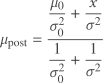
The posterior imply of μ is
This equation turns into extra comprehensible once we introduce precisons τ = 1/σ² and τ0 = 1/σ0².
Then we’ve got
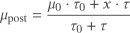
which you’ll learn as saying the posterior imply is the weighted common of the prior imply and x, with the weights given by the precision. Intuitively, you are taking the weighted imply of your conclusions from earlier information and new information, weighting the imply based on how a lot confidence you will have in every.
Beta-binomial mannequin
Now let’s change over to a special information mannequin. Now assume X is a binary random variable, with chance of success p and chance of failure 1 − p, and we assume p has a beta(a, b) distribution.
After observing s successes and f failures, the posterior imply of the distribution on p turns into
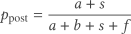
We will rewrite this as
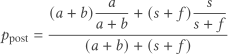
This says that the posterior imply is the weighted common of the prior imply a/(a + b) and the imply of the information s/n. The weights are the prior efficient pattern dimension a + b and the pattern dimension of the brand new information n. On this instance (efficient) pattern dimension is enjoying the position that precision performed within the normal-normal mannequin above.
Gamma-Poisson mannequin
Suppose information have a Poisson distribution with parameter λ, and λ has a gamma(α0, β0) prior distribution [1]. And suppose you observe okay occasions over time t. Then the posterior distribution of λ given the information has a gamma(α0 + okay, β0 + t) prior distribution and the imply of the posterior distribution is given by

As earlier than, the posterior imply is a weighted common of the prior imply and new information, and the weights are interpretable as some type of measure of confidence, particularly time. The variable t is instantly time and the parameter β0 is type of an efficient time, simply as a + b is an efficient pattern dimension for the beta distribution.
Widespread thread
In every instance the posterior imply is the weighted common of the prior imply and the imply of the information, with the weights given by a precision. Nonetheless, precision means one thing totally different in every instance. Within the normal-normal mannequin, precision is the reciprocal of variance, however within the beta-binomial mannequin precision is pattern dimension and within the Poisson-gamma mannequin precision is time.
What all three examples have in widespread is that they’re conjugate fashions utilizing distributions from the “exponential household” of chance distributions. In technical phrases, precision is the multiplicative issue on the ample statistic within the exponent of the posterior kernel.
Associated posts
[1] There are a number of conventions for parameterizing the gamma distribution. Right here we’re utilizing the shape-rate parameterization, the place the imply is α/β.

