

Few days in the past we had a chat by Gergely Neu, who offered his current work:
I am scripting this submit principally to bother him, by presenting this work utilizing tremendous hand-wavy intuitions and cartoon figures. If this is not sufficient, I’ll even discover a technique to point out GANs on this context.
However honestly, I am simply excited as a result of for as soon as, there’s a little little bit of studying concept that I half-understand, no less than at an intuitive stage, because of its reliance on KL divergences and the mutual data.
A easy guessing recreation
Let’s begin this with a easy thought experiment as an instance why and the way mutual data could also be helpful in describing an algorithm’s potential to generalize. Say we’re given two datasets, $mathcal{D}_{practice}$ and $mathcal{D}_{take a look at}$, of the identical dimension for simplicity. We play the next recreation: we each have entry to $mathcal{D}_{practice}$ and $mathcal{D}_{take a look at}$, and we each know what studying algorithm, $operatorname{Alg}$ we will use.
Now I toss a coin and I preserve the consequence (recorded as random variable $Y$) a secret. If it is heads, I run $operatorname{Alg}$ on the coaching set $mathcal{D}_{practice}$. If it is tails, I run $operatorname{Alg}$ on the take a look at knowledge $mathcal{D}_{take a look at}$ as an alternative. I do not inform you which of those I did, I solely divulge to you the ultimate parameter worth $W$. Are you able to guess, simply by $W$, whether or not I skilled on coaching or take a look at knowledge?
For those who can not guess $Y$, that implies that the algorithm returns the identical random $W$ no matter whether or not you practice it on coaching or take a look at knowledge. So the coaching and take a look at losses develop into interchangeable. This suggests that the algorithm will generalize very nicely (on common) and never overfit to the information it is skilled on.
The mutual data, on this case between $W$ and $Y$ quantifies your theoretical potential to guess $Y$ from $W$. The upper this worth is, the better it’s to inform which dataset the algorithm was skilled on. If it is simple to reverse engineer my coin toss from parameters, it implies that the algorithm’s output could be very delicate to the enter dataset it is skilled on. And that probably implies poor generalization.
Notice by: an algorithm generalizing nicely on common doesn’t suggest it really works nicely on common. It simply implies that there will not be a big hole between the anticipated coaching and anticipated take a look at error. Take for instance an algorithm returns a randomly initialized neural community, with out even touching the information. That algorithm generalizes extraordinarily nicely on common: it does simply as poorly on take a look at knowledge because it does on coaching knowledge.
Illustrating this in additional element
Under is an illustration of my thought experiment for SGD.
Within the high row, I doodled the distribution of the parameter $W_t$ at varied timesteps $t=0,1,2,ldots,T$ of SGD. We begin the algorithm by initializing $W$ randomly from a Gaussian (left panel). Then, every stochastic gradient replace modifications the distribution of $W_t$ a bit in comparison with the distribution of $W_{t-1}$. How the form of the distribution modifications depends upon the information we use within the SGD steps. Within the high row, for instance I ran SGD on $mathcal{D}_{practice}$ and within the backside, I run it on $mathcal{D}_{take a look at}$. The distibutions $p(W_tvert mathcal{D})$ I drew right here describe the place the SGD iterate is prone to be after $t$ steps of SGD began from random initialization. They aren’t to be confused with Bayesian posteriors, for instance.
We all know that working the algorithm on the take a look at set would produce low take a look at error. Subsequently, sampling a weight vector $W$ from $p(W_Tvert mathcal{D}_{take a look at})$ could be nice if we may do this. However in follow, we won’t practice on the take a look at knowledge, all we’ve the flexibility to pattern from is $p(W_Tvert mathcal{D}_{practice})$. So what we would like for good generalization, is that if $p(W_Tvert mathcal{D}_{take a look at})$ and $p(W_Tvert mathcal{D}_{practice})$ had been as shut as potential. The mutual data between $W_T$ and my coinflip $Y$ measures this closeness by way of the Jensen-Shannon divergence:
$$
mathbb{I}[Y, W_T] = operatorname{JSD}[p(W_Tvert mathcal{D}_{test})|p(W_Tvert mathcal{D}_{train})]
$$
So, in abstract, if we are able to assure that the ultimate parameter an algorithm comes up with does not reveal an excessive amount of details about what dataset it was skilled on, we are able to hope that the algorithm has good generalization properties.
Mutual Inforrmation-based Generalization Bounds
These obscure intuitions will be formalized into actual information-theoretic generalization bounds. These had been first offered in a basic context in (Russo and Zou, 2016) and in a extra clearly machine studying context in (Xu and Raginsky, 2017). I will give a fast – and presumably considerably handwavy – overview of the principle outcomes.
Let $mathcal{D}$ and $mathcal{D}’$ be random datasets of dimension $n$, drawn i.i.d. from some underlying knowledge distribution $P$. Let $W$ be a parameter vector, which we get hold of by working a studying algorithm $operatorname{Alg}$ on the coaching knowledge $mathcal{D}$: $W = operatorname{Alg}(mathcal{D})$. The algorithm could also be non-deterministic, i.e. it could output a random $W$ given a dataset. Let $mathcal{L}(W, mathcal{D})$ denote the lack of mannequin $W$ on dataset $mathcal{D}$. The anticipated generalization error of $operatorname{Alg}$ is outlined as follows:
$$
textual content{gen}( operatorname{Alg}, P) = mathbb{E}_{mathcal{D}sim P^n,mathcal{D}’sim P^n, Wvert mathcal{D}sim operatorname{Alg}(mathcal{D})}[mathcal{L}(W, mathcal{D}’) – mathcal{L}(W, mathcal{D})]
$$
If we unpack this, we’ve two datasets $mathcal{D}$ and $mathcal{D}’$, the previous taking the function of the coaching dataset, the latter of the take a look at knowledge. We take a look at the anticipated distinction between the coaching and take a look at losses ($mathcal{L}(W, mathcal{D})$ and $mathcal{L}(W, mathcal{D}’)$), the place $W$ is obtained by working $operatorname{Alg}$ on the coaching knowledge $mathcal{D}$. The expectation is taken over all potential random coaching units, take a look at units, and over all potential random outcomes of the educational algorithm.
The data theoretic sure states that for any studying algorithm, and any loss operate that is bounded by $1$, the next inequality holds:
$$
gen(operatorname{Alg}, P) leq sqrt{frac{mathbb{I}[W, mathcal{D}]}{n}}
$$
The principle time period within the RHS of this sure is the mutual infomation between the coaching knowledge mathcal{D} and the pararmeter vector $W$ the algorithm finds. It basically quantifies the variety of bits of knowledge the algorithm leaks concerning the coaching knowledge into the parameters it learns. The decrease this quantity, the higher the algorithm generalizes.
Why we won’t apply this to SGD?
The issue with making use of these good, intuitive bounds to SGD is that SGD, in truth, leaks an excessive amount of details about the precise minibatches it’s skilled on. Let’s return to my illustrative instance of getting to guess if we ran the algorithm on coaching or take a look at knowledge. Take into account the state of affairs the place we begin type some parameter worth $w_t$ and we replace both with a random minibatch of coaching knowledge (blue) or a random minibatch of take a look at knowledge (orange).
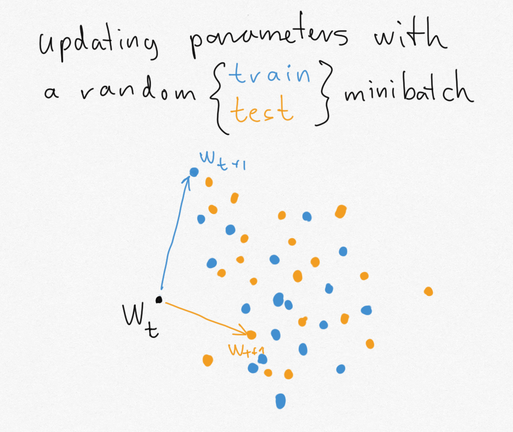
For the reason that coaching and take a look at datasets are assumed to be of finite dimension, there are solely a finite variety of potential minibatches. Every of those minibatches can take the parameter to a singular new location. The issue is, the set of areas you may attain with one dataset (blue dots) doesn’t overlap with the set of areas you may attain when you replace with the opposite dataset (orange dots). Out of the blue, if I offer you $w_{t+1}$, you may instantly inform if it is an orange or blue dot, so you may instantly reconstruct my coinflip $Y$.
Within the extra basic case, the issue with SGD within the context of information-theoretic bounds is that the quantity of knowledge SGD leaks concerning the dataset it was skilled on is excessive, and in some instances could even be infinite. That is really associated to the issue that a number of of us seen within the context of GANs, the place the true and faux distributions could have non-overlapping help, making the KL divergence infinite, and saturating out the Jensen-Shannon divergence. The primary trick we got here up with to resolve this downside was to easy issues out by including Gaussian noise. Certainly, including noise is essential what researches have been doing to use these information-theoretic bounds to SGD.
Including noise to SGD
The very first thing folks did (Pensia et al, 2018) is to review a loud cousin of SGD: stochastic gradient Langevin dynamics (SGLD). SGDL is like SGD however in every iteration we add a little bit of Gaussian noise to the parameters along with the gradient replace. To grasp why SGLD leaks much less data, take into account the earlier instance with the orange and blue level clouds. SGLD makes these level clouds overlap by convolving them with Gaussian noise.
Nonetheless, SGLD just isn’t precisely SGD, and it is not likely used as a lot in follow. In an effort to say one thing about SGD particularly, Neu (2021) did one thing else, whereas nonetheless counting on the thought of including noise. As an alternative of baking the noise in as a part of the algorithm, Neu solely provides noise as a part of the evaluation. The algorithm being analysed continues to be SGD, however after we measure the mutual data we’ll measure the mutual data between $mathbb{I}[W + xi; mathcal{D}]$, the place $xi$ is Gaussian noise.
I depart it to you to take a look at the small print of the paper. Whereas the findings fall in need of explaining whether or not SGD have any tendency to seek out options that generalise nicely, a few of the outcomes are good and interpretable: they join the generalization of SGD to the noisiness of gradients in addition to the smoothness of the loss alongside the precise optimization path that was taken.