Making a shiny as an instance the TWFE steady weights

Brantly Callaway, Andrew Goodman-Bacon and Pedro Sant’Anna (hereafter CBS) have a brand new article conditionally accepted at American Financial Assessment on steady remedy difference-in-differences. The paper has three major components:

• an introduction and formalization of varied causal parameters associated to a remedy “dosage” acceptable for the difference-in-differences framework. This isn’t what I’ll talk about at the moment.

• an introduction of an estimator that one can use to estimate a few of these causal parameters when you could have a steady remedy dosage and a difference-in-differences remedy project. That isn’t what I’ll talk about at the moment both.

• a decomposition of conventional two-way mounted results (TWFE) estimator utilizing Frisch-Waugh-Lovell. That is what I’ll discuss at the moment.

There are 4 decompositions within the paper, and at the moment I’ll solely discuss certainly one of them: the degrees. Within the final substack on this, I labored by that one.

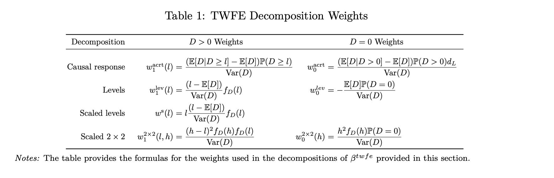
Right here it’s formally:

And so with all that out of the best way, I’ll transfer on to the subsequent merchandise on my agenda which is to make use of Claude Code to create a shiny app that helps all of us higher perceive simply what’s going on in that formulation. I’ve a stroll by of that right here in a 35 minute video, which resulted on this shiny app that you need to use now that will help you higher perceive the TWFE decomposition and the whereabouts of unfavourable weights that it makes use of to calculate its coefficients. That is my first shiny app, and technically Claude Code made it so it isn’t even my shiny app, however I assumed it was enjoyable. I’m internet hosting it on my web site.

There it’s! My new CBS shiny app for the extent decomposition. Let me show you how to navigate it. First, discover there are 4 tables labeled Stage, Scaled degree, Causal response and Scaled 2×2. For those who click on on the others, they’ve a “Coming quickly” web page. The one working proper now’s the Stage one as that’s the one one to date we now have mentioned.

The photographs on the backside are from the deck:

Let me briefly stroll you thru it. There are a number of components in every of the decompositions and this slide illustrates them:

The issues on the left are the load components and the issues on the correct are the actual decomposition. So we’re doing degree weight, and subsequently we now have three components to it: the imply of the remedy dosage within the knowledge (E[D]), the variance, and the density. We combine over the doses utilizing the density formulation. Keep in mind our TWFE formulation from earlier:

There are two items inside this weight — the load related to models which have zero dose, and people who have constructive dose. Look carefully at Desk 1, row 2, labeled “Ranges” and also you’ll see it.

Again to the components. Right here’s the primary one: the imply, E[D]:

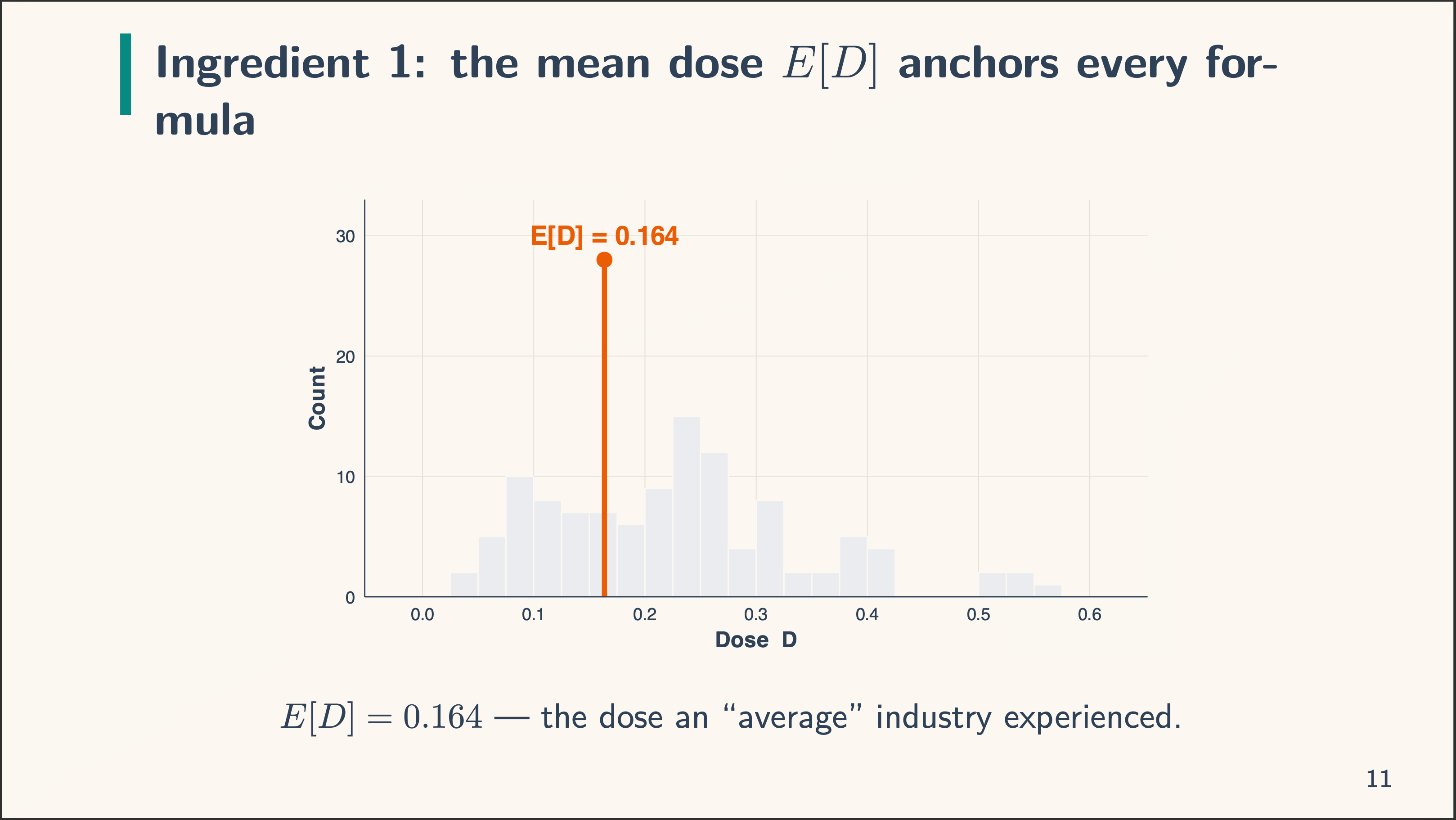
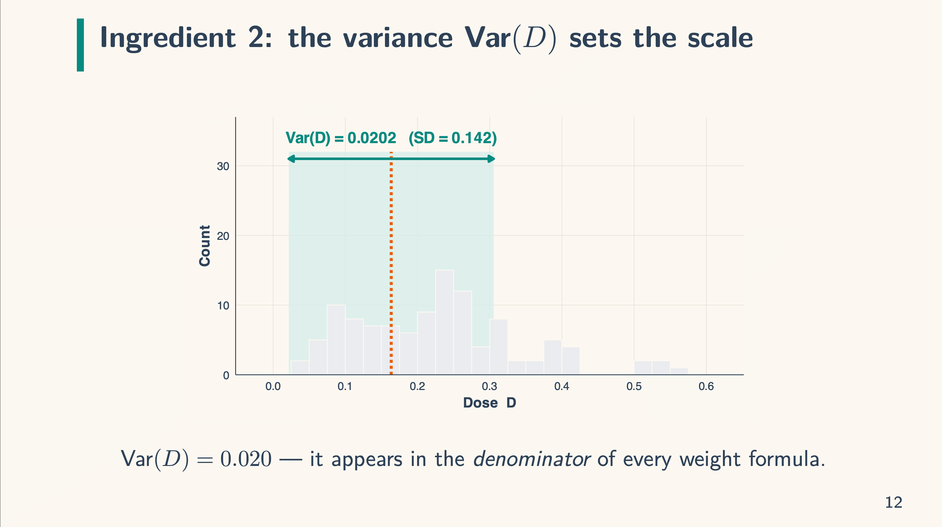
Discover that on this case the imply dose (a tariff on this case) is 0.164. We are going to dangle on to that. Then there may be the variance. The variance recall is the sq. of the usual deviation measuring the unfold of the dose across the imply we simply recognized. And it is the same as 0.0202, or 0.02 for brief. The variance scales the load and seems within the denominator.

After which there may be the density, f_D(l). That is what we will probably be integrating over. The dosage is introduced as steady, but when it was multi-valued, we’d simply take weighted averages. When the density is excessive, there are various models with that worth and when it’s low, there are few. The truth that it’s excessive at zero within the picture under implies that there are a lot of models with zero dose. After we work with the density formulation, we calculate the density at a given dose, l. So if the dose was l=0.10, we simply calculate the density related to it.

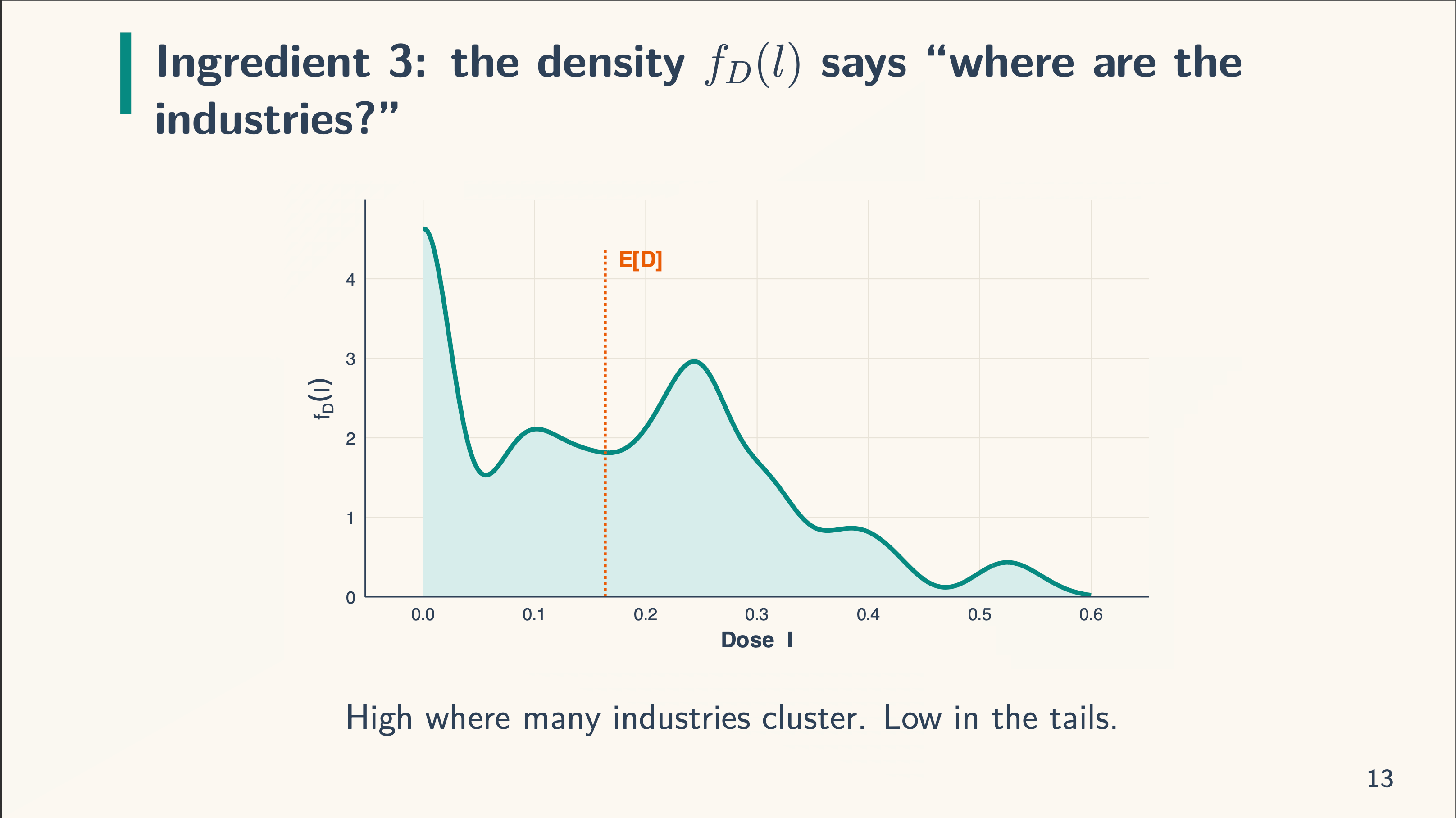
And simply to make sure all of us see it, the x-axis all the time has the dose. The y-axis has the frequency, or depend, or variety of models, within the first two components, and the density within the third.

Alright, so let’s look once more actual fast on the shiny app web page for the extent decomposition. As an illustration, let’s say I need to know the density at 0.365. That’s, for industries with the tariff worth of 0.365, what’s the density worth? I merely slide the slider button on the highest left labeled “Dose l:” to 0.365. And spot, it routinely calculates it. The worth of the density at that time is 0.834. You’ll be able to see it on the far proper of the “Six components” formulation, and it’s also possible to see that it populates the picture labeled “Plug within the numbers on the chosen l”.

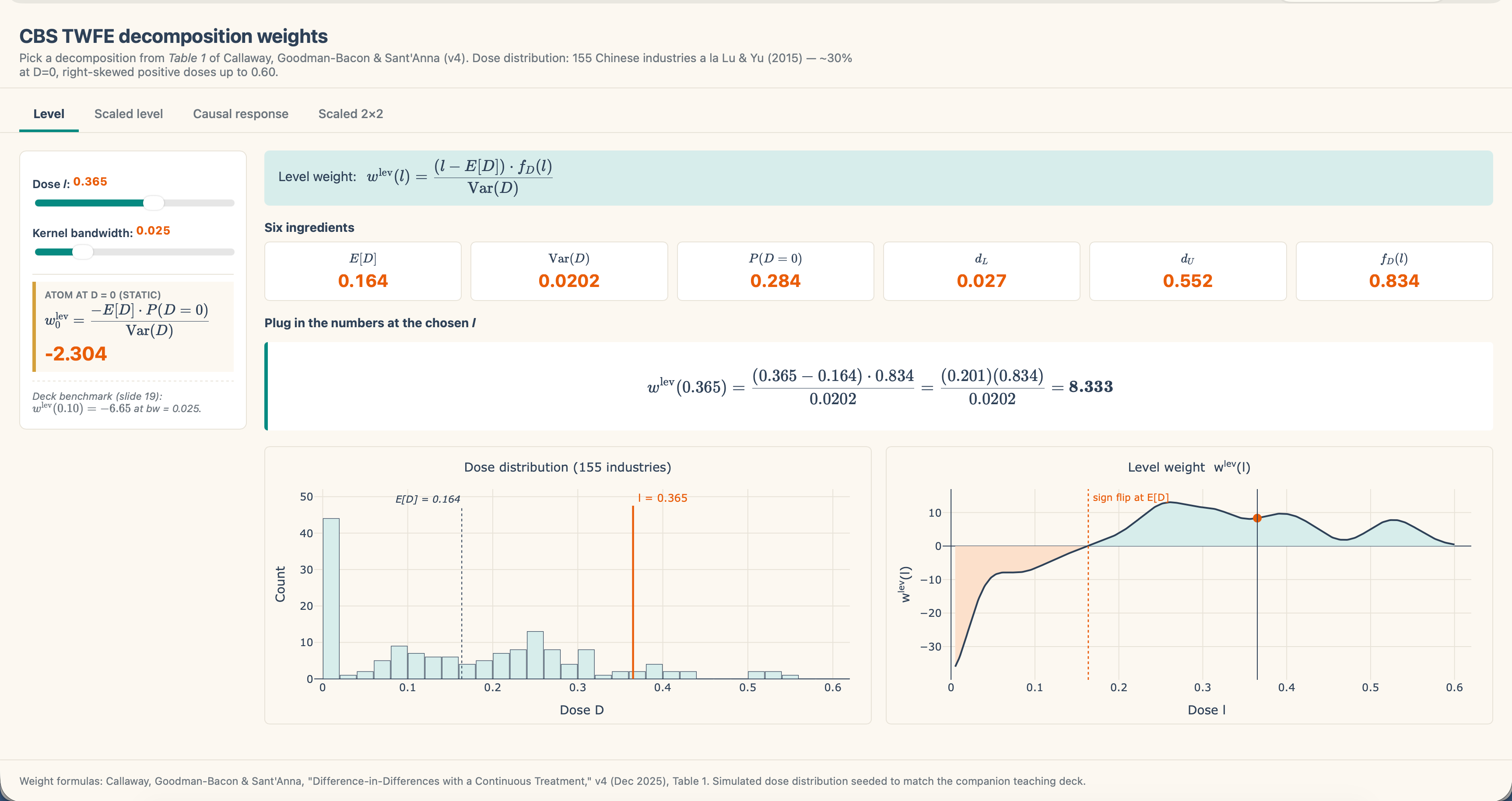
And so given the imply of 0.165, the variance of 0.0202 and a density worth (which not like the imply and variance just isn’t a continuing however modifications at every dose) of 0.834, we get:

And that’s it! That’s how the extent formulation works. You’ll be able to both transfer the slider left and proper to search out every business’s density worth, or you’ll be able to transfer your cursor over the density and that’ll present you the density related to that dosage. Both manner. However the formulation stays the identical.

Now essentially the most fascinating factor on this decomposition is the signal flip. Discover what occurs when the dosage is precisely equal to the imply. The imply, recall, is E[D], equalling 0.164:

So, when you could have a unit or set of models whose dose is precisely the imply, then the load on them curiously is zero. Now in our case, as a result of the remedy is a steady dose for which the likelihood of any actual worth is zero, I don’t present the load at that degree as there isn’t a one with precisely the imply dose. However, you’ll be able to see what occurs if you happen to transfer the slider left and proper — when industries have an above common dose, they’re positively weighted, however once they have a under common dose, they’re negatively weighted. For example this, I filmed myself a second time.

Within the above video, I really had a discrepancy which took me a bit to grasp. Claude had minimal dosage at 0.027 and a most dosage of 0.552. However the Gaussian kernel smeared a bit likelihood mass to the left of the smallest noticed dose. So the kernel put a teeny tiny little bit of density at 0.005. The load is technically computable however substantively empty — it’s a weight on a dose group with no industries in it.

So within the new one, you’ll nonetheless see the signal flip, however now there are vertical dashed strains on the lowest to highest doses. It isn’t within the video, however if you happen to watch the video, you’ll discover that’s the place I begin to notice it. I believe it was most likely effective to have left it there, however I felt just like the smoothing that the kernel perform was doing was complicated me, and subsequently I modified it. The highest panel makes use of a kernel smoother of 0.005, however the backside one was a bit underneath the most important kernel smoothing worth doable. Simply so you’ll be able to see.

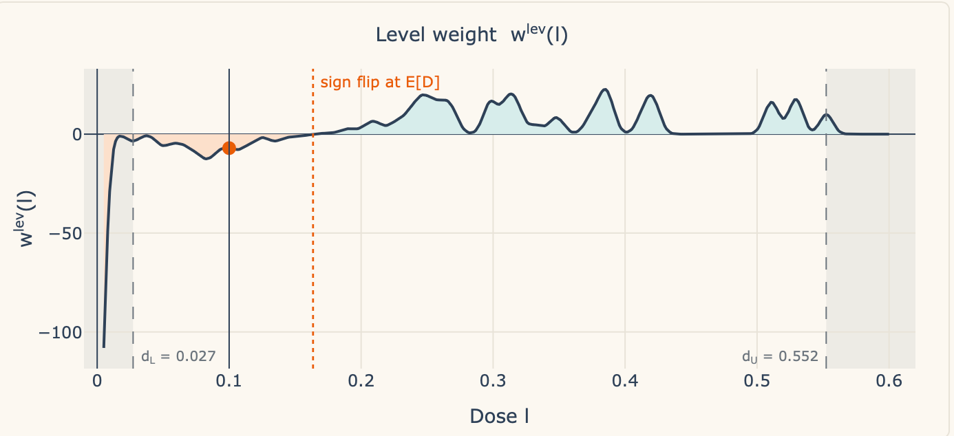
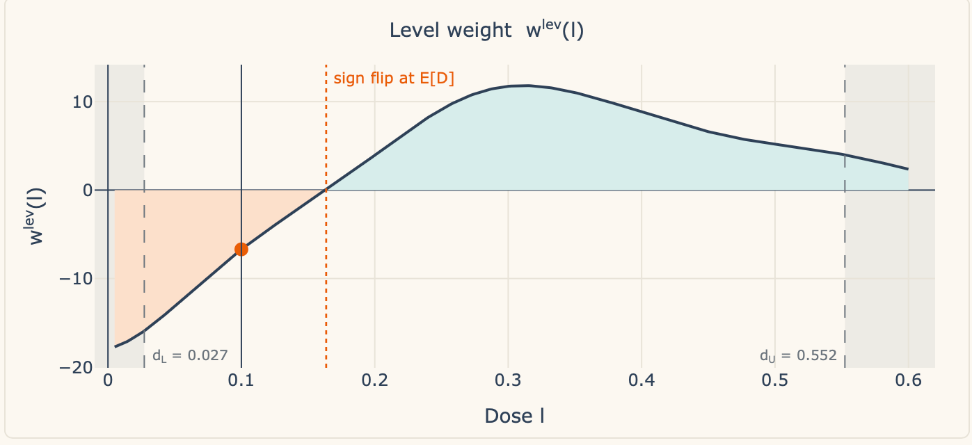
Anyway, the TWFE estimator integrates from the smallest to highest doses, and when industries have doses under the imply, we’re in that zone to the left in that sort of orange hue-ish trying vary, all of that are unfavourable weights, and when the dose is above the imply, we’re above zero in that turquoise blue and that’s constructive weights.

And there you go! That’s the shiny app, plus two video walk-throughs, the primary one which you need to use to higher see how you can use Claude Code to make a shiny app, and the second was strolling you thru deciphering the shiny app. I hope you discovered this useful! Each for utilizing Claude Code to make a shiny app, and for deciphering the TWFE decomposition while you’re regression is in its “degree” formulation (which is able to most likely be more often than not tbh).

And naturally, if you happen to discovered this handy, think about changing into a paying subscriber!