

Most wearable well being fashions are constructed one final result at a time. That strategy breaks down at thirty-five endpoints. Labels are costly and retrospective annotation is infeasible.
Google Analysis launched SensorFM, a basis mannequin for wearable well being pre-trained on greater than 1 trillion minutes of sensor knowledge from 5 million folks.
What’s SensorFM?
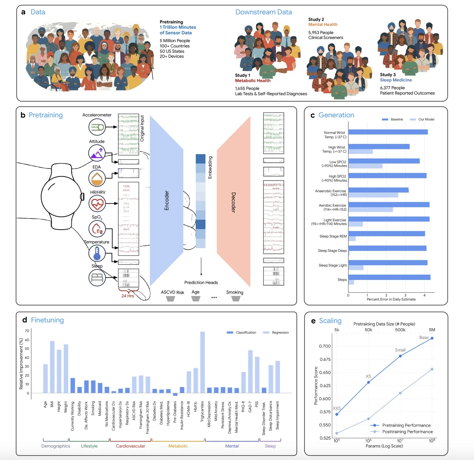
SensorFM is a Giant Sensor basis Mannequin for wearable time-series illustration studying. It ingests 34 one-minute mixture options drawn from 5 sensors: PPG, accelerometer, EDA, pores and skin temperature, and altimeter. These options are organized into seven classes, over a 24-hour context window.
The spine is a ViT-1D encoder skilled with a masked-autoencoder goal and a patch dimension of [20, 1]. Pretraining used 5,000,000 consented members, sampled between September 2024 and September 2025. That corpus spans 100+ international locations, all 50 U.S. states, and 20+ Fitbit and Pixel Watch fashions. It totals over two billion hours, or multiple trillion minutes.
4 variants exist, every paired with a proportional knowledge quantity.
| Variant | Parameters | Encoder hidden / layers | Proportional knowledge | Sensor-hours |
|---|---|---|---|---|
| XXS | 138,740 | 64 / 2 | 5K topics | 2×10⁶ |
| XS | 933,204 | 128 / 4 | 50K topics | 2×10⁷ |
| S | 7,290,068 | 256 / 8 | 500K topics | 2×10⁸ |
| B | 110,763,412 | 768 / 12 | 5M topics | 2×10⁹ |
Analysis makes use of separate knowledge. It covers 13,985 topics throughout three potential IRB-approved research. These are metabolic, cardiac and respiratory well being (N = 1,655), sleep (N = 6,377), and psychological well being (N = 5,953). The 35 duties cowl cardiovascular (6), metabolic (8), psychological well being (8), sleep (3), demographics (4), and way of life (6).
The Scaling Case
With that setup, the primary query is whether or not scale buys something measurable. The analysis crew swept 4 mannequin sizes in opposition to 4 knowledge volumes.
SensorFM-B on the 5M corpus cuts reconstruction validation loss by 31% versus SensorFM-XXS. Generative loss drops 28% on common. Downstream, it beneficial properties ΔAUC = 0.09 on classification and Δr = 0.21 on regression. Throughout variants, B wins 33 of 35 duties, and XXS ranks final on 33 of 35.
The failure case is equally informative. SensorFM-B skilled on solely 5K topics posts a 1.082 validation loss. That’s worse than each smaller variant on the similar quantity. Pretraining was stopped early as a result of the mannequin overfit.
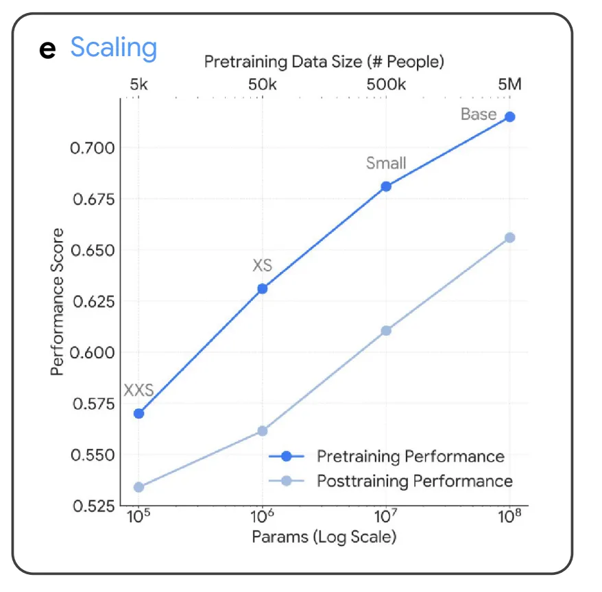
Consequently, all headline outcomes assume knowledge volumes scaled proportionally to capability. Alongside that co-scaled diagonal, imply ROC AUC strikes .664, .681, .710, .752. Imply Pearson r strikes .386, .435, .536, .612. The above determine reveals the development has not saturated.
AIM: Dealing with Lacking Knowledge as Sign
Scaling alone doesn’t clarify these numbers. Actual streams fragment throughout charging, off-wrist durations, and power-saving modes. Standard strategies both impute the gaps, injecting bias, or drop the home windows, discarding knowledge.
SensorFM as a substitute makes use of Adaptive and Inherited Masking (AIM), launched by Xu et al. in LSM-2. The utilized masks is the union of the inherited missingness masks and the factitious masks. Loss is computed solely on artificially masked patches that had floor fact. Two-stage token masking, utilizing token dropout and a focus masking, retains this environment friendly.
As a result of the decoder learns to reconstruct ablated observations, imputation and forecasting come at no cost.
| Generative job | Imply fill | NN fill | Linear interp. | SensorFM-B |
|---|---|---|---|---|
| Random imputation, 80% | 0.915 | 1.020 | 0.854 | 0.215 |
| Temporal interpolation, 60 min | 0.904 | 0.943 | 0.777 | 0.468 |
| Temporal extrapolation, 60 min | 0.937 | 1.102 | 1.102 | 0.563 |
| Sign imputation, 12/26 channels | 1.025 | 1.025 | 1.025 | 0.170 |
Reconstruction MSE on the held-out take a look at set, decrease is healthier.
In opposition to the very best baseline, SensorFM improves random imputation by 74.8%. Sensor sign imputation improves by 83.7%.
Fingers-On: Adapting the Embeddings
Turning that illustration into predictions is simple. The encoder stays frozen. Embeddings are aggregated per particular person, utilizing the imply and customary deviation throughout days. These cut back to 50 principal parts. A linear head then trains underneath five-fold, person-independent cross-validation.
import numpy as np
from sklearn.decomposition import PCA
from sklearn.linear_model import LogisticRegression
from sklearn.model_selection import StratifiedKFold
from sklearn.metrics import roc_auc_score

def person_level(emb, pid):
    """Collapse day-level embeddings into one vector per participant."""
    folks = np.distinctive(pid)
    feats = []
    for p in folks:
        e = emb[pid == p]                    # (n_days, d)
        feats.append(np.concatenate([e.mean(axis=0), e.std(axis=0)]))
    return np.nan_to_num(np.stack(feats)), folks   # pandas std() is NaN at 1 day

X, folks = person_level(emb, pid)           # emb: frozen SensorFM embeddings
y = labels[people]                           # one label per participant

aucs = []
for tr, te in StratifiedKFold(5, shuffle=True, random_state=0).break up(X, y):
    pca = PCA(n_components=50).match(X[tr])    # PCA-50, match on the practice fold solely
    clf = LogisticRegression(max_iter=400)   # paper: AdamW, lr 5e-3, wd 1e-4, 400 steps
    clf.match(pca.rework(X[tr]), y[tr])
    p = clf.predict_proba(pca.rework(X[te]))[:, 1]
    aucs.append(roc_auc_score(y[te], p))
print(np.imply(aucs))
This linear probe beats a supervised feature-engineered baseline on 34 of 35 duties. Chosen outcomes observe.
| Job | Metric | Demos. solely | Feat. Eng. | SensorFM-B |
|---|---|---|---|---|
| Age | r | – | .662 | .920 |
| Psychological Well being Med. | ROC | .594 | .773 | .819 |
| PHQ-8 | r | .303 | .354 | .450 |
| Insulin Resistance | ROC | .717 | .710 | .761 |
| Hypertension Dx | ROC | .762 | .747 | .786 |
| Framingham 30 Danger | r | .782 | .592 | .714 |
The final row will not be an outlier. ASCVD and Framingham scores are calculated from demographic options. Demographic-only fashions due to this fact win by building. The analysis crew reviews SensorFM finest on 31 of 35 duties, not all of them.
Two caveats sit in the identical tables. Demographics nonetheless assist SensorFM on 22 of 30 duties, although the carry shrinks with scale. In very-low-label regimes, demographic priors alone stay sturdy.
The Agentic Classroom
Even a linear probe wants per-task tuning. To automate that, the analysis crew ran a ‘classroom’ of 5 LLM scholar brokers. These span gemini-2.5 flash by means of gemini-3.1 professional preview. Brokers generate, execute, rating, and refine Python heads over 20 cycles, utilizing unreduced embeddings.
In complete they ran 30,516 experiments. Agent-found heads beat the linear probe on 16 of 20 classification duties, measured by F1. Additionally they raised Pearson correlation on 12 of 15 regression duties. Answer high quality tracked the Synthetic Evaluation Intelligence Index.
The successful options are conservative. Nearly all lowered the embedding house to 50–100 dimensions. Linear fashions outnumbered non-linear ones, and ensembles appeared in underneath 1 / 4.
Grounding a Private Well being Agent
The ultimate experiment checks SensorFM as a device, not a benchmark entry. Gemini 3 Flash generated well being summaries for 31 actual participant profiles. Each situation obtained demographics and feature-engineered each day metrics. Circumstances then added SensorFM predictions, ground-truth targets, or nothing.
In response to the analysis paper, 4 board-certified physicians, blinded to situation, produced 1,860 rankings throughout 5 rubric dimensions. Including SensorFM predictions beat the baseline total (W = 10110, p < 0.001), and on every dimension. Its predictions have been statistically indistinguishable from floor fact (p = 0.396).
Use Circumstances
- Screening and danger stratification: A frozen encoder plus one linear head flags candidates for confirmatory lab work. The paper scopes this to screening, not analysis.
- Repairing each day summaries: With 60 contiguous minutes ablated, SensorFM retains 99.7% step-count and 99.9% deep-sleep accuracy.
- Label-scarce research: Probe frozen embeddings as a substitute of coaching end-to-end. Examine in opposition to a demographics-only baseline first.
- Grounded teaching: The agent immediate forbids emitting uncooked regression values or boolean flags. Predictions are interpreted qualitatively as a substitute.
Interactive Explorer
Have to associate with us for selling your GitHub Repo OR Hugging Face Web page OR Product Launch OR Webinar and many others.? Join with us

