

Monitoring lineages of the Omicron variant of the SARS-CoV-2 virus continues to be an necessary well being consideration. The World Well being Group identifies BA.1, BA.1.1, and the latest BA.2 as the commonest sublineages. A latest examine from Japan, Yamasoba et al. (2022), compares, amongst different traits, the transmissibility of those three Omicron lineages with the most recent Delta variant. It identifies BA.2 to have the best transmissibility of the 4. Preprint of the examine is obtainable at bioarxiv.org. One fascinating side of the examine is the applying of Bayesian multilevel fashions for representing lineage development dynamics. On this publish, I show the right way to use Stata’s bayesmh and bayesstats abstract instructions to carry out related evaluation.
The datasets can be found at github.com. The information had been compiled from the GISAID database, https://www.gisaid.org/hcov19-variants/, on February 1, 2022.
Observations on the variety of instances for every lineage are collected for 11 nations in a interval of 117 days, from October 1, 2021, to January 25, 2022.
. use omicron_ba2

. summarize

    Variable |        Obs        Imply    Std. dev.       Min        Max
-------------+---------------------------------------------------------
         day |      1,185    58.18312     33.1129          1        117
        yba1 |      1,185    377.2878     1301.07          0      10251
       yba11 |      1,185    168.5561    685.6369          0       7378
        yba2 |      1,185    23.60759    128.7147          0       1481
      ydelta |      1,185     1224.78    2513.555          0      12549
-------------+---------------------------------------------------------
     nation |      1,185     6.03038    3.245177          1         11
The variables yba1, yba11, yba2, and ydelta correspond, respectively, to the variety of instances of BA.1, BA.1.1, and BA.2 lineages and the Delta variant. The variables day and nation establish the day and nation, respectively. The next desk reveals the nation codes and the variety of noticed days for every nation.
| Id | Nation | Days |
| 1 | Austria | 105 |
| 2 | Denmark | 116 |
| 3 | Germany | 116 |
| 4 | India | 117 |
| 5 | Israel | 117 |
| 6 | Philippines | 43 |
| 7 | Singapore | 115 |
| 8 | South Africa | 110 |
| 9 | Swiden | 112 |
| 10 | United Kingdom | 117 |
| 11 | USA | 117 |
For some nations, the info are incomplete. Particularly, for the Philippines, information can be found for less than 43 days, which, as we’ll see later, impacts the evaluation.
Bayesian multilevel multinomial mannequin
In every of the 11 nations, the viral lineages are recorded because the variety of instances on the noticed days. To formally specify the mannequin, allow us to denote variables yba1, yba11, yba2, and ydelta, respectively, as (y_{1ct}), (y_{2ct}), (y_{3ct}), and (y_{4ct}), the place (c) is the nation code and (t) is the commentary time. (y_{lct}) is assumed to comply with a multinomial distribution with whole variety of instances (n_{ct}). The chance of an incidence of a lineage, (theta_{lct}), for lineage (l), nation (c), and time (t) is given by the four-dimensional logistic operate (softmax) utilized to linear features (a_{lc} + b_{lc}occasions t), the place (a_{lc}) and, (b_{lc}) are random-effect parameters.
Extra formally, for lineages (l=1,dots,4) and nations (c=1,dots,11), we now have
$$
y_{lct} sim {rm Multinomial}(n_{ct}, theta_{lct})
theta_{lct} = frac{{rm exp}(mu_{lct})}{sum_{ok=1}^4 {rm exp}(mu_{kct})}hspace{.5cm}
mu_{lct} = a_{lc} + b_{lc} occasions t hspace{1.5cm}
$$
The chance of observing counts (n_1) by way of (n_4), the place (n_1+n_2+n_3+n_4=n_{ct}), is
$$
P(y_{1ct}=n_1, y_{2ct}=n_2, y_{3ct}=n_3, y_{4ct}=n_4) =
frac{n_{ct}!}{n_1!n_2!n_3!n_4!}
theta_{1ct}^{n_1}theta_{2ct}^{n_2}theta_{3ct}^{n_3}theta_{4ct}^{n_4}
$$
For identifiability, I set the random parameters for the BA.1 lineage, (a_{1c}) and (b_{1c}), to 0. On this case, we now have
$$
theta_{1ct} = frac{1}{1+sum_{ok=2}^4 {rm exp}(mu_{kct})}
theta_{2ct} = frac{{rm exp}(mu_{2ct})}{1+sum_{ok=2}^4 {rm exp}(mu_{kct})}
theta_{3ct} = frac{{rm exp}(mu_{3ct})}{1+sum_{ok=2}^4 {rm exp}(mu_{kct})}
theta_{4ct} = frac{{rm exp}(mu_{4ct})}{1+sum_{ok=2}^4 {rm exp}(mu_{kct})}
$$
and the (lct)-observation of the log chances are
$$
{rm const} + y_{2ct}timesmu_{2ct} + y_{3ct}timesmu_{3ct} + y_{4ct}timesmu_{4ct}
hspace{1cm}- n_{ct}occasions{1+{rm exp}(mu_{2ct})+ {rm exp}(mu_{3ct})+ {rm exp}(mu_{4ct})}
$$
For the aim of sampling the posterior mannequin, we are able to ignore the fixed phrases.
The authors suggest Scholar’s (t)-distributions with 6 levels of freedom for the random slope parameters (b_{lc}) to scale back the results of outliers,
$$
b_{lc} sim t_6(beta_l, sigma_l^2)
$$
and flat priors for the random intercepts (a_{lc}) and hyperparameters (beta_l) and (sigma_l^2). As a substitute, to have a correct prior mannequin, I apply weakly informative priors: (N(0, 100)) for random intercepts (a_{lc})s and random slopes (beta_{l})s and ({rm InvGamma}(0.1,0.1)) for the variance parameters (sigma_l^2)s.
To compute the log chance, I outline a brand new variable, ytotal, for the full quantity instances (n_{ct}).
. gen double ytotal = yba1+yba11+yba2+ydelta
As a result of we don’t have a built-in distribution in bayesmh for this chance mannequin, I exploit the llf() choice to specify it in response to the above components. The llf() possibility requires a univariate mannequin specification, so I exploit ytotal as a dependent variable representing the vector of counts ((y_{1ct},y_{2ct},y_{3ct},y_{4ct})).
The linear mixtures (mu_{2ct}), (mu_{3ct}), and (mu_{4ct}) are specified utilizing the outline() possibility. The latter embrace random intercepts A2[country], A3[country], and A4[country] and random slopes B2[country], B3[country], and B4[country]. The random slopes describe the transmissibility of the lineages as compared with BA.1.
To enhance the sampling, I block among the parameters and supply preliminary values inside the area of the posterior.
. bayesmh ytotal, noconstant chance(llf(
>         yba11*{mu2:}+yba2*{mu3:}+ydelta*{mu4:} -
>         ytotal*ln(1+exp({mu2:})+exp({mu3:})+exp({mu4:}))))
>         outline(mu2: A2[country] B2[country]#c.day, noconstant)
>         outline(mu3: A3[country] B3[country]#c.day, noconstant)
>         outline(mu4: A4[country] B4[country]#c.day, noconstant)
>         prior({A2}, regular(0, 100))
>         prior({A3}, regular(0, 100))
>         prior({A4}, regular(0, 100))
>         prior({B2}, t({beta2}, {sigma2}, 6))
>         prior({B3}, t({beta3}, {sigma3}, 6))
>         prior({B4}, t({beta4}, {sigma4}, 6))
>         prior({sigma2 sigma3 sigma4}, igamma(0.1, 0.1) break up)
>         prior({beta2 beta3 beta4}, regular(0, 100) break up)
>         block({beta2 sigma2})
>         block({beta3 sigma3}) block({beta4 sigma4})
>         init({beta2 beta3 beta4} rnormal(1, 1)
>                 {sigma2 sigma3 sigma4} 1) rseed(17)


Burn-in 2500 aaaaaaaaa1000aaaaaaaaa2000aaaaa performed
Simulation 10000 .........1000.........2000.........3000.........4000.........
> 5000.........6000.........7000.........8000.........9000.........10000 performed

Mannequin abstract
------------------------------------------------------------------------------
Probability:
  ytotal ~ logdensity()

Hyperpriors:
  {A2[country] A3[country] A4[country]} ~ regular(0,100)
                          {B2[country]} ~ t({beta2},{sigma2},6)
                          {B3[country]} ~ t({beta3},{sigma3},6)
                          {B4[country]} ~ t({beta4},{sigma4},6)
                 {sigma2 sigma3 sigma4} ~ igamma(0.1,0.1)
                    {beta2 beta3 beta4} ~ regular(0,100)

Expression:
  expr4 : yba11*xb_mu2+yba2*xb_mu3+ydelta*xb_mu4-ytotal*ln(1+exp(xb_mu2)
          +exp(xb_mu3)+exp(xb_mu4))
------------------------------------------------------------------------------

Bayesian regression                              MCMC iterations  =     12,500
Random-walk Metropolis–Hastings sampling         Burn-in          =      2,500
                                                 MCMC pattern dimension =     10,000
                                                 Variety of obs    =      1,185
                                                 Acceptance fee  =      .2528
                                                 Effectivity:  min =     .02015
                                                              avg =     .06866
Log marginal-likelihood                                       max =     .09676

------------------------------------------------------------------------------
             |                                                Equal-tailed
             |      Imply   Std. dev.     MCSE     Median  [95% cred. interval]
-------------+----------------------------------------------------------------
       beta2 |  .0271004     .04504   .001448    .026472  -.0587521   .1217648
      sigma2 |  .0245979   .0132208   .000554   .0207922    .010104   .0613864
       beta3 |  .1527336   .0530795   .001722   .1533625   .0424005   .2561617
      sigma3 |  .0304257   .0174173   .000794   .0260487   .0112527   .0827476
       beta4 | -.1673996   .0474555   .001539  -.1678558  -.2638208  -.0749281
      sigma4 |  .0264834   .0164447   .001159   .0227708    .010781   .0628222
------------------------------------------------------------------------------
There aren’t any apparent convergence points with the mannequin, and the 7% common sampling effectivity for the hyperparameters is sweet.
The constructive estimate for beta2 and beta3 means that BA.1.1 and BA.2 lineages are each extra transmittable than BA.1. Alternatively, the posterior imply estimate for beta4 is damaging, (-0.17), implying much less transmittability of Delta as compared with the unique Omicron BA.1.
Relative efficient replica by nation
The authors of the examine calculate the relative efficient replica quantity in response to the components
$$
r_{lc} = {rm exp}(gammabeta_{lc})
$$
and the common relative efficient replica quantity throughout nations in response to
$$
r_{l} = {rm exp}(gammabeta_{l})
$$
the place (gamma) is the viral technology time, 2.1 days; see Estimating Technology Time of Omicron.
We estimate the replica numbers (r_l) utilizing the bayesstats abstract command. As a result of we assumed BA.1 lineage to be the baseline, the replica numbers are relative to BA.1.
. bayesstats abstract (rba11:exp(2.1*{beta2}))
>         (rba2:exp(2.1*{beta3})) (rdelta:exp(2.1*{beta4}))

Posterior abstract statistics                      MCMC pattern dimension =    10,000

       rba11 : exp(2.1* { beta2 } )
        rba2 : exp(2.1* { beta3 } )
      rdelta : exp(2.1* { beta4 } )

------------------------------------------------------------------------------
             |                                                Equal-tailed
             |      Imply   Std. dev.     MCSE     Median  [95% cred. interval]
-------------+----------------------------------------------------------------
       rba11 |  1.063311   .1011051   .003258   1.057165   .8839283   1.291373
        rba2 |   1.38671   .1545093    .00502   1.379969   1.093126   1.712475
      rdelta |  .7070996   .0705203   .002292   .7029306    .574633   .8544061
------------------------------------------------------------------------------
Based mostly on posterior imply estimates, the replica of BA.1.1 is about 6% larger, BA.2 is about 39% larger, and Delta is about 30% decrease than that of BA.1. These outcomes agree with the findings within the paper that BA.2 has 1.4-fold larger efficient replica than that of BA.1.
Beneath, I present caterpillar plots for the relative efficient replica numbers by nation. Plotted are the posterior imply values together with 95% credible intervals.
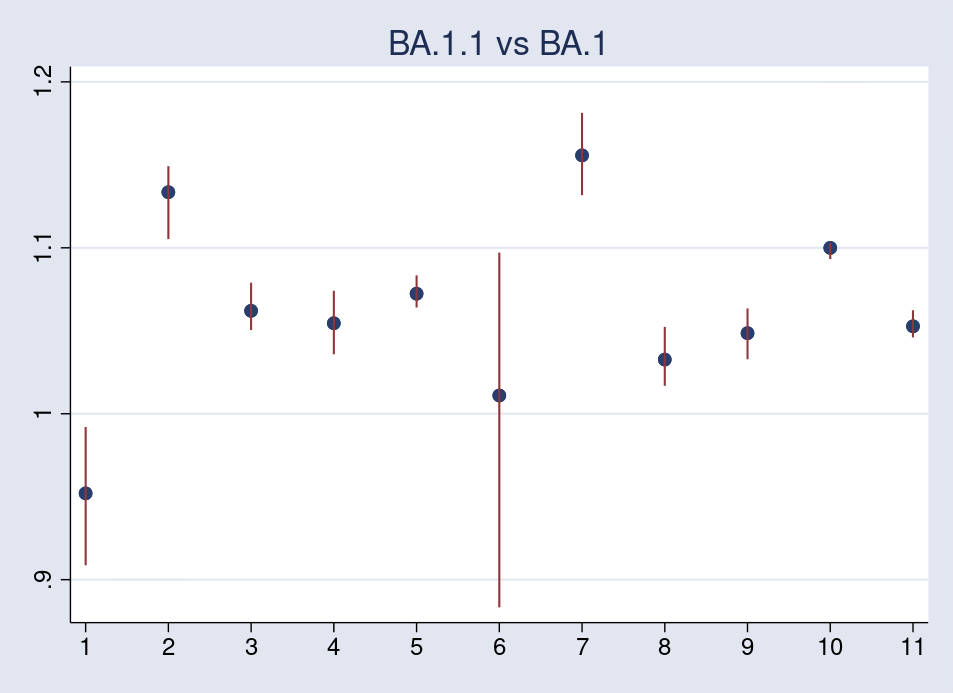
The primary plot compares BA.1.1 with BA.1.
. gen id = mod(_n-1, 11)+1

. quietly bayesstats abstract (exp(2.1*{B2[country]}))

. mat bsum = r(abstract)

. mat bsum = (bsum[1..11,1], bsum[1..11,5], bsum[1..11,6])

. svmat bsum

. twoway scatter bsum1 id || rspike bsum3 bsum2 id, legend(off)
>         xla(1 2 3 4 5 6 7 8 9 10 11, valuelabel) xsc(r(1 11))
>         xtitle("") title("BA.1.1 vs BA.1")

. drop bsum*
All of the values are larger than 1 apart from nation 1, Austria. Additionally obvious is the broad credible interval for nation 6, Philippines, due, in all probability, to the a lot fewer commentary days accessible, solely 43, as compared with the opposite nations, 110 or extra.
The second plot compares BA.2 with BA.1.
. quietly bayesstats abstract (exp(2.1*{B3[country]}))

. mat bsum = r(abstract)

. mat bsum = (bsum[1..11,1], bsum[1..11,5], bsum[1..11,6])

. svmat bsum

. twoway scatter bsum1 id || rspike bsum3 bsum2 id, legend(off)
>         xla(1 2 3 4 5 6 7 8 9 10 11, valuelabel) xsc(r(1 11))
>         xtitle("") title("BA.2 vs BA.1")

. drop bsum*
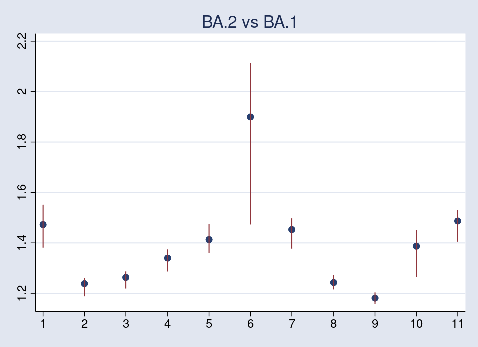
Once more, the replica quantity for the Philippines has larger variability and tends to shift the common across-country replica upward.
The third plot compares Delta with BA.1.
. quietly bayesstats abstract (exp(2.1*{B4[country]}))

. mat bsum = r(abstract)

. mat bsum = (bsum[1..11,1], bsum[1..11,5], bsum[1..11,6])

. svmat bsum

. twoway scatter bsum1 id || rspike bsum3 bsum2 id, legend(off)
>         xla(1 2 3 4 5 6 7 8 9 10 11, valuelabel) xsc(r(1 11))
>         xtitle("") title("Delta vs BA.1")

. drop bsum*
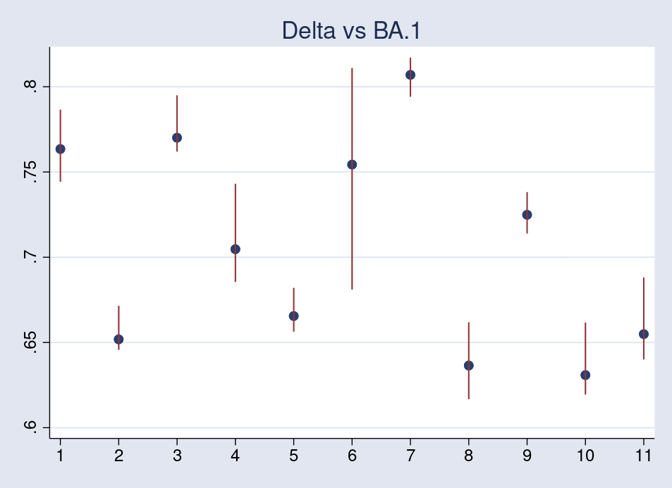
As we’d anticipate, all replica numbers are lower than 1, and the replica quantity for the Philippines has larger variability than the others.
Sensitivity evaluation
The authors of the examine use Scholar’s (t)-prior with 6 levels of freedom for the random slopes (b_{lc}). It’s fascinating to examine whether or not altering the prior impacts the ends in any substantive method.
Beneath, I match fashions utilizing (t)-priors with 2 and 12 levels of freedom for (b_{lc}).
. quietly bayesmh ytotal, noconstant chance(llf(
>         yba11*{mu2:}+yba2*{mu3:}+ydelta*{mu4:} -
>         ytotal*ln(1+exp({mu2:})+exp({mu3:})+exp({mu4:}))))
>         outline(mu2: A2[country] B2[country]#c.day, noconstant)
>         outline(mu3: A3[country] B3[country]#c.day, noconstant)
>         outline(mu4: A4[country] B4[country]#c.day, noconstant)
>         prior({A2}, regular(0, 100))
>         prior({A3}, regular(0, 100))
>         prior({A4}, regular(0, 100))
>         prior({B2}, t({beta2}, {sigma2}, 2))
>         prior({B3}, t({beta3}, {sigma3}, 2))
>         prior({B4}, t({beta4}, {sigma4}, 2))
>         prior({sigma2}{sigma3}{sigma4}, igamma(0.1, 0.1) break up)
>         prior({beta2}{beta3}{beta4}, regular(0, 100) break up)
>         block({beta2}{sigma2})
>         block({beta3}{sigma3}) block({beta4}{sigma4})
>         init({beta2}{beta3}{beta4} rnormal(1, 1)
>                 {sigma2}{sigma3}{sigma4} 1)
>         burnin(5000) rseed(17)

. bayesstats abstract (r2:exp(2.1*{beta2}))
>         (r3:exp(2.1*{beta3})) (r4:exp(2.1*{beta4}))

Posterior abstract statistics                      MCMC pattern dimension =    10,000

          r2 : exp(2.1* { beta2 } )
          r3 : exp(2.1* { beta3 } )
          r4 : exp(2.1* { beta4 } )

------------------------------------------------------------------------------
             |                                                Equal-tailed
             |      Imply   Std. dev.     MCSE     Median  [95% cred. interval]
-------------+----------------------------------------------------------------
          r2 |  1.067439   .0938958   .003041   1.060892   .8874384   1.262244
          r3 |  1.394932   .1392574   .006867   1.381163   1.163633   1.702113
          r4 |   .700393   .0654377   .001962   .6977034   .5754148   .8349086
------------------------------------------------------------------------------

. quietly bayesmh ytotal, noconstant chance(llf(
>         yba11*{mu2:}+yba2*{mu3:}+ydelta*{mu4:} -
>         ytotal*ln(1+exp({mu2:})+exp({mu3:})+exp({mu4:}))))
>         outline(mu2: A2[country] B2[country]#c.day, noconstant)
>         outline(mu3: A3[country] B3[country]#c.day, noconstant)
>         outline(mu4: A4[country] B4[country]#c.day, noconstant)
>         prior({A2}, regular(0, 100))
>         prior({A3}, regular(0, 100))
>         prior({A4}, regular(0, 100))
>         prior({B2}, t({beta2}, {sigma2}, 12))
>         prior({B3}, t({beta3}, {sigma3}, 12))
>         prior({B4}, t({beta4}, {sigma4}, 12))
>         prior({sigma2}{sigma3}{sigma4}, igamma(0.1, 0.1) break up)
>         prior({beta2}{beta3}{beta4}, regular(0, 100) break up)
>         block({beta2}{sigma2})
>         block({beta3}{sigma3}) block({beta4}{sigma4})
>         init({beta2}{beta3}{beta4} rnormal(1, 1)
>                 {sigma2}{sigma3}{sigma4} 1)
>         burnin(5000) rseed(17)

. bayesstats abstract (r2:exp(2.1*{beta2}))
>         (r3:exp(2.1*{beta3})) (r4:exp(2.1*{beta4}))

Posterior abstract statistics                      MCMC pattern dimension =    10,000

          r2 : exp(2.1* { beta2 } )
          r3 : exp(2.1* { beta3 } )
          r4 : exp(2.1* { beta4 } )

------------------------------------------------------------------------------
             |                                                Equal-tailed
             |      Imply   Std. dev.     MCSE     Median  [95% cred. interval]
-------------+----------------------------------------------------------------
          r2 |  1.068262   .1032594    .00325   1.061218   .8759179   1.302069
          r3 |  1.414598     .15648   .005184    1.40231    1.14427   1.765012
          r4 |  .7024785   .0725748   .001915   .6985938    .574165   .8566458
------------------------------------------------------------------------------
I additionally match a mannequin with regular priors for the random slopes.
. quietly bayesmh ytotal, noconstant chance(llf(
>         yba11*{mu2:}+yba2*{mu3:}+ydelta*{mu4:} -
>         ytotal*ln(1+exp({mu2:})+exp({mu3:})+exp({mu4:}))))
>         outline(mu2: A2[country] B2[country]#c.day, noconstant)
>         outline(mu3: A3[country] B3[country]#c.day, noconstant)
>         outline(mu4: A4[country] B4[country]#c.day, noconstant)
>         prior({A2}, regular(0, 100))
>         prior({A3}, regular(0, 100))
>         prior({A4}, regular(0, 100))
>         prior({B2}, regular({beta2}, {sigma2}))
>         prior({B3}, regular({beta3}, {sigma3}))
>         prior({B4}, regular({beta4}, {sigma4}))
>         prior({sigma2}{sigma3}{sigma4}, igamma(0.1, 0.1) break up)
>         prior({beta2}{beta3}{beta4}, regular(0, 100) break up)
>         block({beta2}{sigma2}{beta3}{sigma3}{beta4}{sigma4},
>                 break up gibbs)
>         init({beta2}{beta3}{beta4} rnormal(1, 1)
>                 {sigma2}{sigma3}{sigma4} 1) rseed(17)

. bayesstats abstract (r2:exp(2.1*{beta2}))
>         (r3:exp(2.1*{beta3})) (r4:exp(2.1*{beta4}))

Posterior abstract statistics                      MCMC pattern dimension =    10,000

          r2 : exp(2.1* { beta2 } )
          r3 : exp(2.1* { beta3 } )
          r4 : exp(2.1* { beta4 } )

------------------------------------------------------------------------------
             |                                                Equal-tailed
             |      Imply   Std. dev.     MCSE     Median  [95% cred. interval]
-------------+----------------------------------------------------------------
          r2 |  1.066153   .1080605   .001081   1.061309   .8664183   1.292496
          r3 |  1.405522    .159427   .010062    1.39786   1.120683   1.746765
          r4 |  .7089474    .075455   .000755   .7048609   .5734278   .8714144
------------------------------------------------------------------------------
As evident from the summaries, there aren’t any substantive modifications within the replica quantity estimates, which reveals that our preliminary mannequin is strong to the prior specification of random slopes.
As we noticed above, the replica quantity estimates for the Philippines have excessive variability due to the smaller pattern. It’s fascinating to examine how these estimates change after excluding the Philippines from the estimation pattern.
. quietly bayesmh ytotal if nation != 6, noconstant chance(llf(
>         yba11*{mu2:}+yba2*{mu3:}+ydelta*{mu4:} -
>         ytotal*ln(1+exp({mu2:})+exp({mu3:})+exp({mu4:}))))
>         outline(mu2: A2[country] B2[country]#c.day, noconstant)
>         outline(mu3: A3[country] B3[country]#c.day, noconstant)
>         outline(mu4: A4[country] B4[country]#c.day, noconstant)
>         prior({A2}, regular(0, 100))
>         prior({A3}, regular(0, 100))
>         prior({A4}, regular(0, 100))
>         prior({B2}, t({beta2}, {sigma2}, 6))
>         prior({B3}, t({beta3}, {sigma3}, 6))
>         prior({B4}, t({beta4}, {sigma4}, 6))
>         prior({sigma2}{sigma3}{sigma4}, igamma(0.1, 0.1) break up)
>         prior({beta2}{beta3}{beta4}, regular(0, 100) break up)
>         block({beta2}{sigma2})
>         block({beta3}{sigma3}) block({beta4}{sigma4})
>         init({sigma2}{sigma3}{sigma4} 1)
>         burnin(5000) rseed(17)

. bayesstats abstract (rba11:exp(2.1*{beta2}))
>         (rba2:exp(2.1*{beta3})) (rdelta:exp(2.1*{beta4}))

Posterior abstract statistics                      MCMC pattern dimension =    10,000

       rba11 : exp(2.1* { beta2 } )
        rba2 : exp(2.1* { beta3 } )
      rdelta : exp(2.1* { beta4 } )

------------------------------------------------------------------------------
             |                                                Equal-tailed
             |      Imply   Std. dev.     MCSE     Median  [95% cred. interval]
-------------+----------------------------------------------------------------
       rba11 |  1.101936   .1422373   .006638   1.089014   .8338979   1.415828
        rba2 |  1.313135   .1978823   .006081   1.302977   .9514345   1.731837
      rdelta |  .7242147   .1055362   .010449   .7109377   .5368485   .9596856
------------------------------------------------------------------------------
Now the posterior estimates for the three relative replica numbers all get nearer to 1. Particularly, the replica of BA.2 as compared with BA.1.1, when it comes to posterior imply, drops from 1.4 to 1.3, thus suggesting extra average improve in transmissibility. As well as, the 95% credible intervals for the relative replica of each BA.1.1 and BA.2 now embrace 1.
Reference
Yamasoba, D., I. Kimura, H. Nasser, Y. Morioka, N. Nao, J. Ito, Ok. Uriu, et al. 2022. Virological traits of SARS-CoV-2 BA.2 variant. https://doi.org/10.1101/2022.02.14.480335.