

In this put up I discussed two collection which I denoted t(n) and c(n). The previous is the variety of unlabeled rooted timber with n nodes. The latter is the cumulative sum of the previous, i.e.
The sequence c(n) can also be the variety of constrains on an n-step Runge-Kutta technique; that’s how I turned taken with it.
Now the t(n) sequence has been cataloged as OEIS A000081 and OEIS offers the asymptotic estimate of t(n) for big n as

the place C = 0.4399… and α = 2.9557….
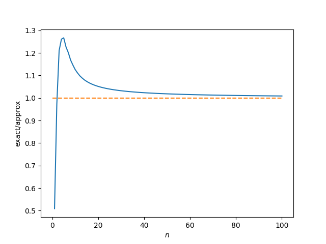
The cumulative sum of t(n), what I’ve referred to as c(n), can also be cataloged in OEIS, sequence quantity A087803. Nevertheless, OEIS doesn’t give an asymptotic estimate for this sequence. I’ll give one right here.
(Replace: After wanting nearer on the web page for A087803 I see that there’s an asymptotic system, the identical one derived right here.)
The premise for my derivation is to imagine the cumulative sum of the asymptotic estimates offers an asymptotic estimate of the cumulative sum. That is justified by the truth that the sequence is rising quickly and solely the previous couple of phrases contribute a lot comparatively to the sum.
The approach illustrated right here can be relevant to the cumulative sum of different collection whose asymptotic kind is thought.
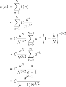
Right here’s code to visualise the speed of convergence.
import numpy as np
import matplotlib.pyplot as plt

# from https://oeis.org/A000081/b000081.txt
A000081 = [
    0,
    1,
    1,
    2,
    4,
    ...
    51384328351659326880337136395054298255277970,
]
A087803 = np.cumsum(A000081)

def approx(n):
    C = 0.43992401257102530
    a = 2.95576528565199497
    return C*a**(n+1)*n**(-3/2)/(a - 1)

n = np.arange(len(A087803))
ratio = A087803/approx(n)

plt.plot(n[1:], ratio[1:])
plt.plot(n, 0*n + 1, '--')
plt.xlabel("$n$")
plt.ylabel("actual/approx")
plt.present()
Right here’s the plot: