

In Customizable tables in Stata 17, half 5, I confirmed you tips on how to use the brand new and improved desk command to create a desk of outcomes from a logistic regression mannequin. We’re more likely to create many extra tables of regression outcomes, and we’ll most likely use the identical model and labels. On this publish, I’ll present you tips on how to save your kinds and labels with the intention to use them to format future tables. I’ll use the Microsoft Phrase doc that we created partly 5 as our aim.
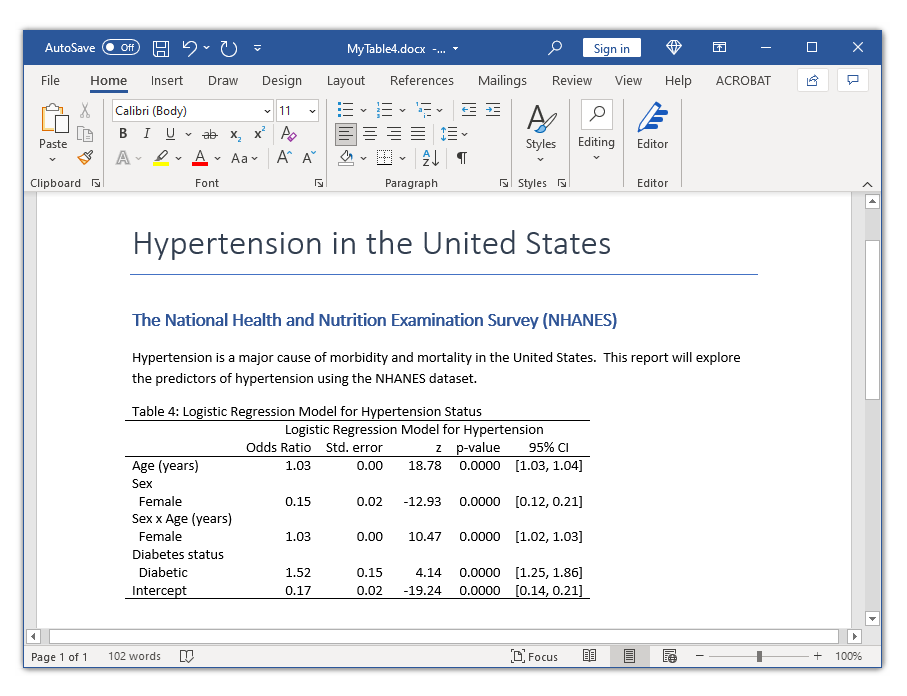
Create the fundamental desk
Let’s start by typing webuse nhanes2l to open the NHANES dataset. Then we’ll use desk to create a primary desk for a logistic regression mannequin for the binary final result highbp. The desk consists of the chances ratios, normal errors, z statistics, p-values, and confidence intervals. Word that I’ve used Stata’s factor-variable notation within the instance beneath to incorporate the primary impact of the continual variable age, the primary results of the explicit variables intercourse and diabetes, and the interplay of age and intercourse.
. webuse nhanes2l
(Second Nationwide Well being and Vitamin Examination Survey)

. desk () (command consequence),
>           command(_r_b _r_se _r_z _r_p _r_ci
>                   : logistic highbp c.age##i.intercourse i.diabetes)

--------------------------------------------------------------------------------------------------
                             |                logistic highbp c.age##i.intercourse i.diabetes
                             |  Coefficient   Std. error        z   p-value          95% CI
-----------------------------+--------------------------------------------------------------------
Age (years)                  |     1.034281     .0018566    18.78     0.000   1.030648    1.037926
Intercourse=Male                     |            1            0
Intercourse=Feminine                   |     .1549363     .0223461   -12.93     0.000   .1167849    .2055511
Intercourse=Male # Age (years)       |            1            0
Intercourse=Feminine # Age (years)     |     1.028856     .0027958    10.47     0.000   1.023391    1.034351
Diabetes standing=Not diabetic |            1            0
Diabetes standing=Diabetic     |     1.521011      .154103     4.14     0.000   1.247073    1.855124
Intercept                    |     .1730928     .0157789   -19.24     0.000    .144772    .2069537
--------------------------------------------------------------------------------------------------
Create and save a customized model
Let’s sort accumulate clear to clear any collections from Stata’s reminiscence.
. accumulate clear
Then we will use the identical accumulate model instructions that we used to format our desk partly 5. I’ve included feedback within the code block beneath to remind us of the aim of every line.
// TURN OFF BASE LEVELS FOR FACTOR VARIABLES
accumulate model showbase off
// STACK THE ROW LEVEL LABELS AND CHANGE THE INTERACTION DELIMITER
accumulate model row stack, delimiter(" x ") nobinder
// REMOVE THE VERTICAL LINE
accumulate model cell border_block, border(proper, sample(nil))
// FORMAT THE NUMBERS
accumulate model cell consequence[_r_b _r_se _r_ci], nformat(%8.2f)
accumulate model cell consequence[_r_p], nformat(%5.4f)
accumulate model cell consequence[_r_ci], sformat("[%s]") cidelimiter(,)
// HIDE THE LOGISTIC REGRESSION COMMAND
accumulate model header command, degree(conceal)
Lastly, we will sort accumulate model save to avoid wasting this model to a file named MyLogitStyle.stjson.
. accumulate model save MyLogitStyle, substitute
(model from mylogit saved to file MyLogitStyle.stjson)
Create and save degree labels
We are able to additionally save customized degree labels. The coefficients in our logistic regression output are literally odds ratios. Partially 5, we used accumulate label ranges to vary the label for the extent _r_b within the dimension consequence from “Coefficient” to “Odds Ratio”.
accumulate label ranges consequence _r_b "Odds Ratio", modify
We are able to use accumulate label save to avoid wasting our customized degree label to a file named MyLogitLabels.stjson.
. accumulate label save MyLogitLabels, substitute
(labels from mylogit saved to file MyLogitLabels.stjson)
Utilizing our saved kinds and labels
We are able to apply our model and labels to a desk utilizing the model() and label() choices once we outline our desk. If you’re in the identical listing the place you simply saved the labels and kinds, you possibly can check with them just by their names. Nonetheless, in case you are in a special listing you possibly can specify the complete path.
. desk () (command consequence),
>          command(_r_b _r_se _r_z _r_p _r_ci
>                  : logistic highbp c.age##i.intercourse i.diabetes)
>          model(c:MyFolderMyLogitStyle.stjson, override)
>          label(c:MyFolderMyLogitLabels.stjson)

-------------------------------------------------------------------------------
                   Odds Ratio   Std. error        z   p-value        95% CI
-------------------------------------------------------------------------------
Age (years)              1.03         0.00    18.78    0.0000   [1.03,    1.04]
Intercourse
  Feminine                 0.15         0.02   -12.93    0.0000   [0.12,    0.21]
Intercourse x Age (years)
  Feminine                 1.03         0.00    10.47    0.0000   [1.02,    1.03]
Diabetes standing
  Diabetic               1.52         0.15     4.14    0.0000   [1.25,    1.86]
Intercept                0.17         0.02   -19.24    0.0000   [0.14,    0.21]
-------------------------------------------------------------------------------
Or, even higher, we will save our kinds and labels the place we will use them anytime. We are able to make our kinds and labels robotically accessible by storing the information in our private ado-directory. You’ll be able to sort sysdir to find your private ado-directory.
. sysdir
   STATA:  C:Program FilesStata17
    BASE:  C:Program FilesStata17adobase
    SITE:  C:Program FilesStata17adosite
    PLUS:  C:UsersChuckStataadoplus
PERSONAL:  c:adopersonal
OLDPLACE:  c:ado
My private ado-directory is c:adopersonal, so I’ll save my model and label information in that folder.
. accumulate model save "c:adopersonalMyLogitStyle", substitute
(model from mylogit saved to file c:adopersonalMyLogitStyle.stjson)

. accumulate label save "c:adopersonalMyLogitLabels", substitute
(labels from mylogit saved to file c:adopersonalMyLogitLabels.stjson)
Now I can use MyLogitStyle and MyLogitLabels anytime to format different tables.
Utilizing our saved kinds and labels with different tables
Let’s clear Stata’s reminiscence and use the Hosmer and Lemeshow low birthweight dataset. We’re excited about predictors of low toddler birthweight (low), outlined as birthweight lower than 2,500 grams.
. webuse lbw, clear
(Hosmer & Lemeshow knowledge)

. describe low age smoke ht

Variable      Storage   Show    Worth
    identify         sort    format    label      Variable label
------------------------------------------------------------------------------------------------------------------------
low             byte    %8.0g                 Birthweight<2500g
age             byte    %8.0g                 Age of mom
smoke           byte    %9.0g      smoke      Smoked throughout being pregnant
ht              byte    %8.0g                 Has historical past of hypertension
Subsequent let’s create a desk for the output of a logistic regression command for the binary dependent variable low. We are able to format our desk utilizing MyLogitStyle and MyLogitLabels.
. desk () (command consequence),
>          command(_r_b _r_se _r_z _r_p _r_ci
>                  : logistic low c.age##i.smoke ht)
>          model(MyLogitStyle, override)
>          label(MyLogitLabels)

----------------------------------------------------------------------------------------------------
                                         Odds Ratio   Std. error       z   p-value        95% CI
----------------------------------------------------------------------------------------------------
Age of mom                                  0.92         0.04   -1.85    0.0646   [0.84,    1.01]
Smoked throughout being pregnant
  Smoker                                       0.36         0.56   -0.66    0.5082   [0.02,    7.37]
Smoked throughout being pregnant x Age of mom
  Smoker                                       1.08         0.07    1.14    0.2542   [0.95,    1.23]
Has historical past of hypertension                    3.47         2.15    2.00    0.0456   [1.02,   11.72]
Intercept                                      2.16         2.27    0.73    0.4642   [0.28,   16.90]
----------------------------------------------------------------------------------------------------
The general format of our desk seems like we anticipated. However the variable labels are too lengthy for our desk.
The row labels in our desk are saved within the dimension colname. We are able to sort accumulate label checklist to view the extent labels.
. accumulate label checklist colname, all

  Assortment: Desk
   Dimension: colname
       Label: Covariate names and column names
Stage labels:
       _cons  Intercept
       _hide
         age  Age of mom
          c1
          c2
          c3
          c4
          ht  Has historical past of hypertension
       smoke  Smoked throughout being pregnant
Let’s use accumulate label ranges to change the labels of the degrees age, ht, and smoke.
. accumulate label ranges colname age "Age", modify

. accumulate label ranges colname ht "Hypertension", modify

. accumulate label ranges colname smoke "Smoke", modify
Now we will sort accumulate preview to verify our work.
. accumulate preview

-------------------------------------------------------------------------
              Odds Ratio   Std. error       z   p-value        95% CI
-------------------------------------------------------------------------
Age                 0.92         0.04   -1.85    0.0646   [0.84,    1.01]
Smoke
  Smoker            0.36         0.56   -0.66    0.5082   [0.02,    7.37]
Smoke x Age
  Smoker            1.08         0.07    1.14    0.2542   [0.95,    1.23]
Hypertension        3.47         2.15    2.00    0.0456   [1.02,   11.72]
Intercept           2.16         2.27    0.73    0.4642   [0.28,   16.90]
-------------------------------------------------------------------------
Word that we nonetheless used accumulate to customise our desk, despite the fact that we did many of the work with our saved kinds and labels.
Conclusion
On this publish, we discovered tips on how to use accumulate model save and accumulate label save to avoid wasting our customized kinds and labels. We additionally discovered tips on how to apply these customized kinds and labels to different tables. Stata has many predefined kinds, and you may study extra about them within the handbook.
The power to avoid wasting and reuse customized kinds and labels permits us to streamline and automate our workflow for creating paperwork. For instance, many individuals in educational settings submit manuscripts for publication in educational journals. They’ll create customized codecs and labels that meet every journal’s necessities and apply them to their manuscripts. Folks in enterprise or authorities settings might report the identical info to totally different organizations, and so they can save customized kinds and labels for every report. Investing the time to create customized kinds and layouts pays dividends in saved time later.
That is the ultimate publish I had deliberate for the “Customizable tables in Stata 17” collection. My aim was to elucidate the fundamentals of the brand new desk and accumulate instructions, present you just a few helpful examples, and show how you should utilize these instruments to create your personal customized tables. I hope I’ve achieved that aim, and I’ve had a lot enjoyable that I’d not rule out future posts on this subject!