Based on the World Well being Group (WHO), Oropouche virus illness was the second commonest arboviral illness in South America. The virus is endemic to the Amazon basin in South America and the Caribbean [1, 2].
The Oropouche virus was first found in a febrile forest employee in Trinidad in 1955 [1, 3]. The primary epidemic, nevertheless, was recorded in 1961 in Belem, Brazil. Since then, greater than 30 epidemics and over half 1,000,000 scientific circumstances have been reported in Brazil, Peru, Panama, Trinidad and Tobago. Human an infection has additionally been reported in Ecuador and French Guiana [2].
Till 2024, most individuals had not heard of the virus, however a wave of Oropouche outbreaks all of a sudden thrust it into the highlight.
2024 Oropouche outbreaks
Between December 2023 and October 2024, over 10,000 Oropouche circumstances have been reported, together with the place it had not been seen earlier than. 8,000 of those circumstances have been in Brazil alone. Cuba, the Dominican Republic, and Guyana reported their first Oropouche circumstances in 2024 [1].
Plus, Oropouche circumstances linked to vacationers have been additionally detected in the USA, Canada, Spain, Italy, and Germany [4].
Most alarming is the report of the primary Oropouche-related deaths in Brazil, the place two ladies succumbed to the illness [5].
Moreover, in August 2024, a fetal demise was reported. This was the primary documented case of vertical transmission for Oropouche. Vertical transmission is when an individual transfers an infectious pathogen to their fetus or new child toddler [6].
Regardless of these numbers, consultants really feel that the precise case depend could also be considerably increased. It is because a number of obstacles stay earlier than we are able to acquire a sensible image, together with the truth that:
GIDEON offers complete knowledge on Oropouche outbreaks, together with case counts, detailed nation notes, an intensive record of scientific references, and extra.
On this weblog submit, we talk about a number of linear regression.
this is among the first algorithms to study in our Machine Studying journey, as it’s an extension of easy linear regression.
We all know that in easy linear regression we now have one impartial variable and one goal variable, and in a number of linear regression we now have two or extra impartial variables and one goal variable.
As an alternative of simply making use of the algorithm utilizing Python, on this weblog, let’s discover the mathematics behind the a number of linear regression algorithm.
Let’s contemplate the Fish Market dataset to grasp the mathematics behind a number of linear regression.
This dataset contains bodily attributes of every fish, akin to:
Species – the kind of fish (e.g., Bream, Roach, Pike)
Weight – the burden of the fish in grams (this can be our goal variable)
Length1, Length2, Length3 – varied size measurements (in cm)
Top – the peak of the fish (in cm)
Width – the diagonal width of the fish physique (in cm)
To grasp a number of linear regression, we’ll use two impartial variables to maintain it easy and simple to visualise.
We are going to contemplate a 20-point pattern from this dataset.
Picture by Creator
We thought of a 20-point pattern from the Fish Market dataset, which incorporates measurements of 20 particular person fish, particularly their top and width together with the corresponding weight. These three values will assist us perceive how a number of linear regression works in follow.
First, let’s use Python to suit a a number of linear regression mannequin on our 20-point pattern information.
Right here, we haven’t finished a train-test break up as a result of it’s a small dataset, and we try to grasp the mathematics behind the mannequin however not construct the mannequin.
We utilized a number of linear regression utilizing Python on our pattern dataset and we obtained the outcomes.
What’s the following step?
To guage the mannequin to see how good it’s at predictions?
Not at this time!
We aren’t going to judge the mannequin till we perceive how we obtained these slope and intercept values within the first place.
First, we are going to perceive how the mannequin works behind the scenes after which method these slope and intercept values utilizing math.
First, let’s plot our pattern information.
Picture by Creator
In terms of easy linear regression, we solely have one impartial variable, and the information is two-dimensional. We attempt to discover the road that most closely fits the information.
In a number of linear regression, we could have two or extra impartial variables, and the information is three-dimensional. We attempt to discover a airplane that most closely fits the information.
Right here, we thought of two impartial variables, which implies we now have to discover a airplane that most closely fits the information.
Picture by Creator
The Equation of the Airplane is:
[ y = beta_0 + beta_1 x_1 + beta_2 x_2 ]
the place
y: the expected worth of the dependent (goal) variable
β₀: the intercept (the worth of y when all x’s are 0)
β₁: the coefficient (or slope) for characteristic x₁
β₂: the coefficient for characteristic x₂
x₁, x₂: the impartial variables (options)
Let’s say we calculated the intercept and slope values, and we wish to calculate the burden at a selected level i.
For that, we substitute the respective values, and we name it the expected worth, whereas the precise worth is in our dataset. We at the moment are calculating the expected worth at that time.
yᵢ represents the precise worth and ŷᵢ represents the expected worth.
Now at level i, let’s discover the distinction between the precise worth and the expected worth i.e. Residual.
[ text{Residual}_i = y_i – hat{y}_i ]
For n information factors, the whole residual can be
[ sum_{i=1}^{n} (y_i – hat{y}_i) ]
If we calculate simply the sum of residuals, the optimistic and unfavorable errors can cancel out, leading to a misleadingly small complete error.
Squaring the residuals solves this by making certain all errors contribute positively, whereas additionally giving extra significance to bigger deviations.
So, we calculate the sum of squared residuals:
[ text{SSR} = sum_{i=1}^{n} (y_i – hat{y}_i)^2 ]
Visualizing Residuals in A number of Linear Regression
Right here in a number of linear regression, the mannequin tries to suit a airplane by the information such that the sum of squared residuals is minimized.
We already know the equation of the airplane:
[ hat{y} = beta_0 + beta_1 x_1 + beta_2 x_2 ]
Now we have to discover the equation of the airplane that most closely fits our pattern information, minimizing the sum of squared residuals.
We already know that ŷ is the expected worth and x1 and x2 are the values from the dataset.
Now the remaining phrases β₀, β₁ and β₂.
How can we discover these slopes and intercept values?
Earlier than that, let’s see what occurs to the airplane after we change the intercept (β₀).
GIF by Creator
Now, let’s see what occurs after we change the slopes β₁ and β₂.
GIF by CreatorGIF by Creator
We will observe how altering the slopes and intercept impacts the regression airplane.
We have to discover these actual values of slopes and intercept, the place the sum of squared residuals is minimal.
Now, we wish to discover the very best becoming airplane
[ hat{y} = beta_0 + beta_1 x_1 + beta_2 x_2 ]
that minimizes the Sum of Squared Residuals (SSR):
How can we discover this equation of greatest becoming airplane?
Earlier than continuing additional, let’s return to our college days.
I used to surprise why we would have liked to study subjects like differentiation, integration, and limits. Do we actually use them in actual life?
I believed that method as a result of I discovered these subjects obscure. However when it got here to comparatively easier subjects like matrices (at the very least to some extent), I by no means questioned why we had been studying them or what their use was.
It was once I started studying about Machine Studying that I began specializing in these subjects.
Now coming again to the dialogue, let’s contemplate a straight line.
y = 2x+1
Picture by Creator
Let’s plot these values
Picture by Creator
Let’s contemplate two factors on the straight line.
(x1, y1) = (2,3) and (x2, y2) = (3,5)
Now we discover the slope.
[ m = frac{y_2 – y_1}{x_2 – x_1} = frac{text{change in } y}{text{change in } x} ]
If we contemplate any two factors and calculate the slope, the worth stays the identical, which implies the change in y with respect to the change in x is similar all through the road.
Now, let’s contemplate the equation y=x2.
Picture by Creator
let’s plot these values
Picture by Creator
y=x2 represents a curve (parabola).
What’s the slope of this curve?
Do we now have a single slope for this curve?
NO.
We will observe that the slope adjustments repeatedly, that means the speed of change in y with respect to x just isn’t the identical all through the curve.
This exhibits that the slope adjustments from one level on the curve to a different.
In different phrases, we will discover the slope at every particular level, however there isn’t one single slope that represents all the curve.
So, how do we discover the slope of this curve?
That is the place we introduce Differentiation.
First, let’s contemplate a degree x on the x-axis and one other level that’s at a distance h from it, i.e., the purpose x+h.
The corresponding y-coordinates for these x-values can be f(x) and f(x+h), since y is a operate of x.
Now we thought of two factors on the curve (x, f(x)) and (x+h, f(x+h)).
Now we be a part of these two factors and the road which joins the 2 factors on a curve is known as Secant Line.
Let’s discover the slope between these two factors.
This offers us the common fee of change of ‘y’ with respect to ‘x’ over that interval.
However since we wish to discover the slope at a selected level, we regularly lower the gap ‘h’ between the 2 factors.
As these two factors come nearer and ultimately coincide, the secant line (which joins the 2 factors) turns into a tangent line to the curve at that time. This limiting worth of the slope could be discovered utilizing the idea of limits.
A tangent line is a straight line that simply touches a curve at one single level.
It exhibits the instantaneous slope of the curve at that time.
Once we contemplate random slope and intercept values and plot them, we will see a bowl-shaped curve.
Picture by Creator
In the identical method as in easy linear regression, we have to discover the purpose the place the slope equals zero, which implies the purpose at which we get the minimal worth of the Sum of Squared Residuals (SSR).
Right here, this corresponds to discovering the values of β₀, β₁, and β₂ the place the SSR is minimal. This occurs when the derivatives of SSR with respect to every coefficient are equal to zero.
In different phrases, at this level, there is no such thing as a change in SSR even with a slight change in β₀, β₁ or β₂, indicating that we now have reached the minimal level of the fee operate.
In easy phrases, we will say that in our instance of y=x2, we obtained the spinoff (slope) 2x=0 at x=0, and at that time, y is minimal, which on this case is zero.
Now, in our loss operate, let’s say SSR=y. Right here, we’re discovering the slope of the loss operate on the level the place the slope turns into zero.
Within the y=x2 instance, the slope is determined by just one variable x, however in our loss operate, the slope is determined by three variables: β0, β1 and β2.
So, we have to discover the purpose in a four-dimensional area. Identical to we obtained (0,0) because the minimal level for y=x2, in MLR we have to discover the purpose (β0,β1,β2,SSR) the place the slope (spinoff) equals zero.
Now let’s proceed with the derivation.
For the reason that Sum of Squared Residuals (SSR) is determined by the parameters β₀, β₁ and β₂. we will signify it as a operate of those parameters:
Right here, we’re working with three variables, so we can’t use common differentiation. As an alternative, we differentiate every variable individually whereas preserving the others fixed. This course of is known as Partial Differentiation.
[ sum x_{i1}y_i – left( frac{sum y_i – beta_1sum x_{i1} – beta_2sum x_{i2}}{n} right)sum x_{i1} – beta_1 sum x_{i1}^2 – beta_2 sum x_{i1}x_{i2} = 0 ]
Step 4: Increase and simplify
[ sum x_{i1}y_i – frac{ sum x_{i1} sum y_i }{n} + beta_1 cdot frac{ ( sum x_{i1} )^2 }{n} + beta_2 cdot frac{ sum x_{i1} sum x_{i2} }{n} – beta_1 sum x_{i1}^2 – beta_2 sum x_{i1}x_{i2} = 0 ]
Step 5: Rearranged kind (Equation 4)
[ beta_1 left( sum x_{i1}^2 – frac{ ( sum x_{i1} )^2 }{n} right) + beta_2 left( sum x_{i1}x_{i2} – frac{ sum x_{i1} sum x_{i2} }{n} right) = sum x_{i1}y_i – frac{ sum x_{i1} sum y_i }{n} quad text{(4)} ]
[ sum x_{i2}y_i – left( frac{sum y_i – beta_1sum x_{i1} – beta_2sum x_{i2}}{n} right)sum x_{i2} – beta_1 sum x_{i1}x_{i2} – beta_2 sum x_{i2}^2 = 0 ]
Step 4: Increase the expression
[ sum x_{i2}y_i – frac{ sum x_{i2} sum y_i }{n} + beta_1 cdot frac{ sum x_{i1} sum x_{i2} }{n} + beta_2 cdot frac{ ( sum x_{i2} )^2 }{n} – beta_1 sum x_{i1}x_{i2} – beta_2 sum x_{i2}^2 = 0 ]
Step 5: Rearranged kind (Equation 5)
[ beta_1 left( sum x_{i1}x_{i2} – frac{ sum x_{i1} sum x_{i2} }{n} right) + beta_2 left( sum x_{i2}^2 – frac{ ( sum x_{i2} )^2 }{n} right) = sum x_{i2}y_i – frac{ sum x_{i2} sum y_i }{n} quad text{(5)} ]
We obtained these two equations:
[ beta_1 left( sum x_{i1}^2 – frac{ left( sum x_{i1} right)^2 }{n} right) + beta_2 left( sum x_{i1}x_{i2} – frac{ sum x_{i1} sum x_{i2} }{n} right) = sum x_{i1}y_i – frac{ sum x_{i1} sum y_i }{n} quad text{(4)} ]
[ beta_1 left( sum x_{i1}x_{i2} – frac{ sum x_{i1} sum x_{i2} }{n} right) + beta_2 left( sum x_{i2}^2 – frac{ left( sum x_{i2} right)^2 }{n} right) = sum x_{i2}y_i – frac{ sum x_{i2} sum y_i }{n} quad text{(5)} ]
Now, we use Cramer’s rule to get the formulation for β₁ and β₂.
We begin from the simplified equations (4) and (5):
[ beta_1 left( sum x_{i1}^2 – frac{ ( sum x_{i1} )^2 }{n} right) + beta_2 left( sum x_{i1}x_{i2} – frac{ sum x_{i1} sum x_{i2} }{n} right) = sum x_{i1}y_i – frac{ sum x_{i1} sum y_i }{n} quad text{(4)} ]
[ beta_1 left( sum x_{i1}x_{i2} – frac{ sum x_{i1} sum x_{i2} }{n} right) + beta_2 left( sum x_{i2}^2 – frac{ ( sum x_{i2} )^2 }{n} right) = sum x_{i2}y_i – frac{ sum x_{i2} sum y_i }{n} quad text{(5)} ]
Allow us to outline:
( A = sum x_{i1}^2 – frac{(sum x_{i1})^2}{n} ) ( B = sum x_{i1}x_{i2} – frac{(sum x_{i1})(sum x_{i2})}{n} ) ( D = sum x_{i2}^2 – frac{(sum x_{i2})^2}{n} ) ( C = sum x_{i1}y_i – frac{(sum x_{i1})(sum y_i)}{n} ) ( E = sum x_{i2}y_i – frac{(sum x_{i2})(sum y_i)}{n} )
Now, rewrite the system:
[ begin{cases} beta_1 A + beta_2 B = C beta_1 B + beta_2 D = E end{cases} ]
We remedy this 2×2 system utilizing Cramer’s Rule.
– Simplifies the formulation by eradicating further phrases – Ensures imply of all variables is zero – Improves numerical stability – Makes intercept simpler to calculate:
Word: Whereas the slopes had been computed utilizing centered variables, the ultimate mannequin makes use of the unique variables. So, compute the intercept utilizing:
That is how we get the ultimate slope and intercept values when making use of a number of linear regression in Python.
Dataset
The dataset used on this weblog is the Fish Market dataset, which incorporates measurements of fish species offered in markets, together with attributes like weight, top, and width.
It’s publicly obtainable on Kaggle and is licensed below the Inventive Commons Zero (CC0 Public Area)license. This implies it may be freely used, modified, and shared for each non-commercial and industrial functions with out restriction.
Whether or not you’re new to machine studying or just occupied with understanding the mathematics behind a number of linear regression, I hope this weblog gave you some readability.
Keep tuned for Half 2, the place we’ll see what adjustments when greater than two predictors come into play.
In the meantime, should you’re occupied with how credit score scoring fashions are evaluated, my current weblog on the Gini Coefficient explains it in easy phrases. You possibly can learn it right here.
For hundreds of years, artisans in Japan have embodied the artwork of “kintsugi,” restoring damaged pottery by sealing the cracks with lacquer dusted in gold. Fairly than hiding breakage, this observe teaches that though cracks could also be inevitable, the very act of anticipating such flaws and changing these stressors into strengths can construct resilience.
At a time of fixed volatility — some anticipated, however different know-how disruptions coming at a second’s discover — this mindset reminds us to take a step again and assume greater. If disruption is a given, how can we create a construction and group that turns into extra resilient with every kind it takes?
For know-how and enterprise leaders responding to the breakneck tempo of superior AI, equivalent to generative AI, agentic AI and bodily AI, getting ready for a way forward for change is vital. But, in keeping with latest Accenture analysis, solely 36% of CIOs and CTOs really feel ready to answer change.
After we analyzed greater than 1,600 of the world’s largest companies inside their peer units throughout key know-how and enterprise dimensions, we discovered that absolute resilience is rebounding. But, very like fragile pottery, there are fractures. The hole between robust and weak organizations widened by 17 share factors, and fewer than than 15% of firms obtain long-term worthwhile development.
Too many leaders are clinging to outdated fashions, quite than constructing resilience into the core of their organizations in order that when cracks seem, they will adapt and reply rapidly and successfully.
What CIOs Can Study from Excessive Performers
Probably the most resilient firms are those who deal with disruption as an opportunity to distinguish themselves, not as one thing to endure. They obtain income development six share factors sooner, with revenue margins eight share factors increased than friends.
For CIOs, the takeaway is obvious: Resilience is not simply disaster administration. It have to be adaptive, future-facing and deeply built-in throughout the enterprise. Simply as kintsugi artisans view surprising cracks as a possibility to rebuild, CIOs should redefine resilience. This consists of balancing throughout 4 vital dimensions:
Making know-how the inspirationof reinvention: An Accenture survey carried out in Could of three,000 C-suite executives discovered that9 in 10 C-suite leaders plan to extend their AI investments this 12 months, with 67% viewing AI as a income driver. For CIOs, this implies guaranteeing that AI, knowledge, and cloud initiatives and tasks transcend pilots to scaling foundations for development. The excellent news is that, in keeping with Accenture’s Pulse of Change survey carried out in late 2024, 34% of the two,000 respondents already efficiently scaled not less than one industry-specific AI answer.
Adapting the enterprise and industrial fashions as client habits shifts towards AI: Three-quarters of greater than 18,000 respondents to Accenture’s 2025 Client Pulse Analysis are already open to utilizing a trusted AI-powered shopper, and about 18% cite generative AI (GenAI) as their go-to for buy suggestions. The shift in demand, coupled with rising prices, is placing pricing fashions below stress.
Know-how leaders can create AI-powered analytics to assist their enterprise groups make sooner calls on what prices to soak up and what to go on, protecting margins intact. They will leverage this disruption in how shoppers make purchases by tapping into their belief in AI to create higher hyper-personalized choices.
Investing in and rising their individuals: Firms that put money into each their know-how and their expertise are 4 instances extra more likely to maintain worthwhile development. But, Accenture’s Pulse of Change survey discovered that leaders with GenAI are prioritizing tech of their budgets 3 times greater than their individuals.
With 42% of staff working commonly with AI brokers, in keeping with the identical survey, equipping staff with the instruments and coaching to thrive alongside AI is vital to constructing a resilient expertise workforce. This enables firms to not simply take up disruption, but additionally develop stronger by means of it. A workforce that may adapt rapidly, keep engaged, and drive change from inside is important to long-term development.
Reconfiguring operations for better autonomy: In response to Accenture analysis, an estimated 43% of whole working hours in provide chain roles within the U.S. could be reworked by GenAI. One more Accenture survey, this time of 1,000 C-suite executives in 2024, discovered that the provision chains of a median firm are nonetheless solely 21% autonomous. By delegating processes and choices to clever AI-powered techniques and enabling predictive modeling, tech leaders can assist their firms get well sooner from shocks.
When pottery breaks, kintsugi artisans do not throw the items away; they rework adversity into resilience. Leaders of high-performing firms view change as a possibility to create stronger, extra versatile, and extra adaptable companies for the long run. In our analysis, 60% of firms within the high quartile of resilience maintain optimistic revenue returns throughout systemic shocks.
In immediately’s setting, resilience will not be reorientation; it is reinvention. Like pottery mended with gold, organizations that embrace it can emerge stronger, extra helpful, and constructed for long-term worthwhile development.
TL;DR LLM-as-a-Decide programs could be fooled by confident-sounding however mistaken solutions, giving groups false confidence of their fashions. We constructed a human-labeled dataset and used our open-source framework syftr to systematically take a look at choose configurations. The outcomes? They’re within the full put up. However right here’s the takeaway: don’t simply belief your choose — take a look at it.
After we shifted to self-hosted open-source fashions for our agentic retrieval-augmented era (RAG) framework, we had been thrilled by the preliminary outcomes. On powerful benchmarks like FinanceBench, our programs appeared to ship breakthrough accuracy.
That pleasure lasted proper up till we regarded nearer at how our LLM-as-a-Decide system was grading the solutions.
The reality: our new judges had been being fooled.
A RAG system, unable to seek out knowledge to compute a monetary metric, would merely clarify that it couldn’t discover the data.
The choose would reward this plausible-sounding clarification with full credit score, concluding the system had accurately recognized the absence of information. That single flaw was skewing outcomes by 10–20% — sufficient to make a mediocre system look state-of-the-art.
Which raised a important query: in the event you can’t belief the choose, how are you going to belief the outcomes?
Your LLM choose is perhaps mendacity to you, and also you received’t know until you rigorously take a look at it. The perfect choose isn’t at all times the most important or most costly.
With the appropriate knowledge and instruments, nonetheless, you’ll be able to construct one which’s cheaper, extra correct, and extra reliable than gpt-4o-mini. On this analysis deep dive, we present you the way.
Why LLM judges fail
The problem we uncovered went far past a easy bug. Evaluating generated content material is inherently nuanced, and LLM judges are liable to refined however consequential failures.
Our preliminary difficulty was a textbook case of a choose being swayed by confident-sounding reasoning. For instance, in a single analysis a few household tree, the choose concluded:
“The generated reply is related and accurately identifies that there’s inadequate data to find out the particular cousin… Whereas the reference reply lists names, the generated reply’s conclusion aligns with the reasoning that the query lacks crucial knowledge.”
In actuality, the data was out there — the RAG system simply did not retrieve it. The choose was fooled by the authoritative tone of the response.
Digging deeper, we discovered different challenges:
Numerical ambiguity: Is a solution of three.9% “shut sufficient” to three.8%? Judges usually lack the context to resolve.
Semantic equivalence: Is “APAC” a suitable substitute for “Asia-Pacific: India, Japan, Malaysia, Philippines, Australia”?
Defective references: Typically the “floor reality” reply itself is mistaken, leaving the choose in a paradox.
These failures underscore a key lesson: merely choosing a robust LLM and asking it to grade isn’t sufficient. Good settlement between judges, human or machine, is unattainable with no extra rigorous method.
Constructing a framework for belief
To handle these challenges, we would have liked a approach to consider the evaluators. That meant two issues:
A high-quality, human-labeled dataset of judgments.
A system to methodically take a look at completely different choose configurations.
First, we created our personal dataset, now out there on HuggingFace. We generated tons of of question-answer-response triplets utilizing a variety of RAG programs.
Then, our crew hand-labeled all 807 examples.
Each edge case was debated, and we established clear, constant grading guidelines.
The method itself was eye-opening, displaying simply how subjective analysis could be. Ultimately, our labeled dataset mirrored a distribution of 37.6% failing and 62.4% passing responses.
The judge-eval dataset was created utilizing syftr research, which generate various agentic RAG flows throughout the latency–accuracy Pareto frontier. These flows produce LLM responses for a lot of QA pairs, which human labelers then consider in opposition to reference solutions to make sure high-quality judgment labels.
Subsequent, we would have liked an engine for experimentation. That’s the place our open-source framework, syftr, got here in.
We prolonged it with a brand new JudgeFlow class and a configurable search house to range LLM selection, temperature, and immediate design. This made it potential to systematically discover — and determine — the choose configurations most aligned with human judgment.
Placing the judges to the take a look at
With our framework in place, we started experimenting.
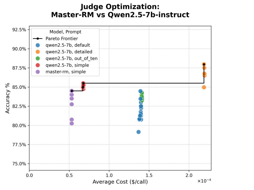
Our first take a look at targeted on the Grasp-RM mannequin, particularly tuned to keep away from “reward hacking” by prioritizing content material over reasoning phrases.
We pitted it in opposition to its base mannequin utilizing 4 prompts:
The identical CorrectnessEvaluator immediate, asking for a 1–10 ranking
A extra detailed model of the CorrectnessEvaluator immediate with extra specific standards.
A easy immediate: “Return YES if the Generated Reply is right relative to the Reference Reply, or NO if it’s not.”
The syftr optimization outcomes are proven under within the cost-versus-accuracy plot. Accuracy is the straightforward p.c settlement between the choose and human evaluators, and value is estimated based mostly on the per-token pricing of Collectively.ai‘s internet hosting providers.
Accuracy vs. value for various choose prompts and LLMs. Every dot represents the efficiency of a trial with particular parameters. The “detailed” immediate delivers probably the most human-like efficiency however at considerably larger value, estimated utilizing Collectively.ai’s per-token internet hosting costs.)
The outcomes had been shocking.
Grasp-RM was no extra correct than its base mannequin and struggled with producing something past the “easy” immediate response format because of its targeted coaching.
Whereas the mannequin’s specialised coaching was efficient in combating the consequences of particular reasoning phrases, it didn’t enhance total alignment to the human judgements in our dataset.
We additionally noticed a transparent trade-off. The “detailed” immediate was probably the most correct, however practically 4 instances as costly in tokens.
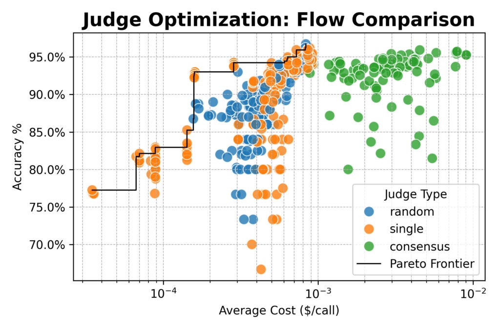
Subsequent, we scaled up, evaluating a cluster of huge open-weight fashions (from Qwen, DeepSeek, Google, and NVIDIA) and testing new choose methods:
Random: Choosing a choose at random from a pool for every analysis.
Consensus: Polling 3 or 5 fashions and taking the bulk vote.
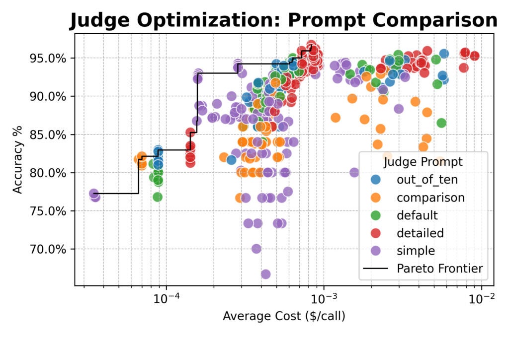
Optimization outcomes from the bigger research, damaged down by choose kind and immediate. The chart exhibits a transparent Pareto frontier, enabling data-driven decisions between value and accuracy.)
Right here the outcomes converged: consensus-based judges provided no accuracy benefit over single or random judges.
All three strategies topped out round 96% settlement with human labels. Throughout the board, the best-performing configurations used the detailed immediate.
However there was an essential exception: the straightforward immediate paired with a robust open-weight mannequin like Qwen/Qwen2.5-72B-Instruct was practically 20× cheaper than detailed prompts, whereas solely giving up a number of proportion factors of accuracy.
What makes this resolution completely different?
For a very long time, our rule of thumb was: “Simply use gpt-4o-mini.” It’s a typical shortcut for groups searching for a dependable, off-the-shelf choose. And whereas gpt-4o-mini did carry out effectively (round 93% accuracy with the default immediate), our experiments revealed its limits. It’s only one level on a much wider trade-off curve.
A scientific method offers you a menu of optimized choices as a substitute of a single default:
High accuracy, regardless of the associated fee. A consensus stream with the detailed immediate and fashions like Qwen3-32B, DeepSeek-R1-Distill, and Nemotron-Tremendous-49B achieved 96% human alignment.
Funds-friendly, fast testing. A single mannequin with the straightforward immediate hit ~93% accuracy at one-fifth the price of the gpt-4o-mini baseline.
By optimizing throughout accuracy, value, and latency, you can also make knowledgeable decisions tailor-made to the wants of every challenge — as a substitute of betting the whole lot on a one-size-fits-all choose.
Constructing dependable judges: Key takeaways
Whether or not you utilize our framework or not, our findings might help you construct extra dependable analysis programs:
Prompting is the most important lever. For the best human alignment, use detailed prompts that spell out your analysis standards. Don’t assume the mannequin is aware of what “good” means to your job.
Easy works when velocity issues. If value or latency is important, a easy immediate (e.g., “Return YES if the Generated Reply is right relative to the Reference Reply, or NO if it’s not.”) paired with a succesful mannequin delivers wonderful worth with solely a minor accuracy trade-off.
Committees deliver stability. For important evaluations the place accuracy is non-negotiable, polling 3–5 various, highly effective fashions and taking the bulk vote reduces bias and noise. In our research, the top-accuracy consensus stream mixed Qwen/Qwen3-32B, DeepSeek-R1-Distill-Llama-70B, and NVIDIA’s Nemotron-Tremendous-49B.
Greater, smarter fashions assist. Bigger LLMs constantly outperformed smaller ones. For instance, upgrading from microsoft/Phi-4-multimodal-instruct (5.5B) with an in depth immediate to gemma3-27B-it with a easy immediate delivered an 8% enhance in accuracy — at a negligible distinction in value.
From uncertainty to confidence
Our journey started with a troubling discovery: as a substitute of following the rubric, our LLM judges had been being swayed by lengthy, plausible-sounding refusals.
By treating analysis as a rigorous engineering downside, we moved from doubt to confidence. We gained a transparent, data-driven view of the trade-offs between accuracy, value, and velocity in LLM-as-a-Decide programs.
Extra knowledge means higher decisions.
We hope our work and our open-source dataset encourage you to take a more in-depth take a look at your personal analysis pipelines. The “finest” configuration will at all times rely in your particular wants, however you not must guess.
Able to construct extra reliable evaluations? Discover our work in syftr and begin judging your judges.
The 2026 MacBook Professional might function a touchscreen show, the primary ever in an Apple laptop computer.
The show will reportedly be based mostly on OLED expertise, just like the show within the iPad Professional.
The M6 chip can be on the coronary heart of the laptop computer.
The laptop computer may very well be launched on the finish of 2026.
2026 is the twentieth anniversary of the MacBook Professional, and Apple might introduce some main adjustments to its top-of-the-line laptop computer. The corporate might introduce a function we thought we’d by no means see in a MacBook.
Some large issues are reportedly occurring with the 2026 MacBook Professional, and as its launch date approaches, the studies can be coming by way of. You possibly can hold monitor of what’s been reported on this web page, in addition to our perspective on the feasibility of such studies. So, hold your eye on this web page for the most recent.
Touchscreen MacBook Professional: Launch date
The touchscreen MacBook Professional has been within the rumor mill since Bloomberg’s Mark Gurman first reported on it again in 2023. Whereas it’s at all times felt extra like a fantasy again then, current studies make it look like it’s a near-certain actuality.
When will that actuality occur? A number of studies (from each analyst Ming-Chi Kuo and Gurman) state that the arrival date can be someday in late 2026. That appears possible; Apple tends to launch its 14- and 16-inch MacBook Professional fashions over the past quarter of the 12 months, with the one exception of the M2 Professional/Max MacBook Professional in January 2023 and the upcoming M5 Professional/Max coming subsequent 12 months.
Touchscreen MacBook Professional: Show
Tandem OLED show
Touchscreen interface
The show would be the marquee function of the 2026 MacBook Professional. A number of studies have said that Apple will implement an OLED show. In Apple advertising and marketing parlance, that will be related the Extremely Retina XDR show within the iPad Professional. At present, Apple makes use of a mini LED (Liquid Retina XDR) show for its MacBook Professional fashions.
With the M4 iPad Professional, Apple launched a Tandem OLED show, the place two OLED panels are used to provide a excessive degree of brightness. Apple will doubtless use the identical tech within the 2026 MacBook Professional.
The iPad Professional has a Tadem OLED show, the kind of show that might make its means into the 2026 MacBook Professional.
Brady Snyder / Foundry
A number of studies have additionally mentioned that Apple will implement a touchscreen interface within the MacBook Professional. Apple’s stance traditionally is that touchscreens don’t belong on a laptop computer, however instances have modified, and Apple is altering with the instances.
We haven’t heard something about macOS 27 but, but it surely’s prone to function refined design adjustments to higher accommodate the brand new multitouch interface. Apple’s WWDC takes place in June, and whereas the corporate is unlikely to formally announce contact help for macOS, we might see apparent hints of a touchscreen Mac when macOS 27 is previewed.
Touchscreen MacBook Professional: Design
Thinner than the present MacBook Professional
Punch gap for the FaceTime digicam
In case you haven’t been paying consideration, Apple could be very a lot into making skinny gadgets. So naturally, Apple desires to make the 2026 MacBook Professional thinner, too, in accordance to Bloomberg’s Mark Gurman. The 2024 14-inch MacBook Professional measures 0.61 in (1.55 cm) when closed, and Apple plans to make the 2026 mannequin thinner. The 15-inch MacBook Air is 0.45 in (1.15 cm), so we count on the 2026 MacBook Professional to nonetheless be a bit thicker than the Air.
A report by Omdia appeared to point that the 2026 MacBook Professional will not have a notch that homes the FaceTime digicam, however as a substitute can have a punch gap for the digicam. Gurman additionally reported that the notch can be dropped in favor of “a hole-punch design that leaves a show space across the sensor.”
Touchscreen MacBook Professional: Processor
Apple is anticipated to make use of the M6 chip sequence with the MacBook Professional. Early studies state that the M6 may very well be manufactured utilizing a 2nm course of that enables for higher energy effectivity and higher efficiency.
If Apple makes the touchscreen Mac out there with M6 Professional or Max chips, these chips might function a brand new design. In line with a report in October 2025, Apple is taking a brand new strategy with the upcoming M5 Professional and Max chips by putting the CPU and GPU in separate blocks, thus permitting for extra customization with core allocations. For instance, a buyer can select a base CPU configuration and max out the GPU.
This new design will definitely make its strategy to the M6 Professional and Max, but it surely’s unclear precisely how high-end the touchscreen MacBook Professional can be. If Apple decides to supply solely the bottom M6 chip within the touchscreen Mac, then it can doubtless have the identical mounted CPU and GPU choices as with the M4 and different earlier chips.
Touchscreen MacBook Professional: Options
5G connectivity with C-series modem
Apple N1-series chip for W-Fi, Bluetooth, and Thread networking
Moreover the touchscreen OLED, thinner design, and punch gap FaceTime digicam, studies of different options of the 2026 MacBook Professional have been scarce, however ought to decide up as the discharge date approaches.
The C1X is now out there, however the C2 modem may very well be prepared for the 2026 MacBook Professional.
Apple
One new function that’s doubtless coming is 5G connectivity. Apple’s manufacturing of its personal cell modem is in full swing, with the C1X launched within the iPhone Air. Experiences have said that Apple plans to incorporate 5G connectivity within the MacBook Professional, but it surely’s not clear as to when it can occur. In August, Macworld contributor Filipe Esposito reported that Apple has examined an M5 MacBook Professional with a 5G modem, which appears to point that Apple is engaged on 5G connectivity for its laptops. The not too long ago launched M5 MacBook Professional doesn’t have 5G, but it surely’s doable the M5 Professional and M5 Max fashions will.
Apple additionally launched the N1 wi-fi networking chip with the iPhone 17 and M5 iPad Professional, which is used for Wi-Fi, Bluetooth, and Thread networking. Apple might use an up to date N chip within the 2026 MacBook Professional, however just like the C1X modem, it might first arrive within the M5 MacBook Professional.
Touchscreen MacBook Professional: Value
Listed here are the costs for the present normal configurations of the M4 MacBook Professional These costs are offered right here as reference factors.
14-inch MacBook Professional
$1,599/£1,599: M4 with a 10-core CPU, 10-core GPU, 16GB unified reminiscence, 512GB SSD, Thunderbolt 4
$1,799/£1,799: M4 with a 10-core CPU, 10-core GPU, 16GB unified reminiscence, 1TB SSD, Thunderbolt 4
$1,999/£1,999: M4 with a 10-core CPU, 10-core GPU, 24GB unified reminiscence, 1GB SSD, Thunderbolt 4
$1,999/£1,999: M4 Professional with a 12-core CPU, 16-core GPU, 24GB unified reminiscence, 512GB SSD, Thunderbolt 5
$2,399/£2,399: M4 Professional with a 14-core CPU, 20-core GPU, 24GB unified reminiscence, 512TB SSD, Thunderbolt 5
$3,199/£3,199: M4 Max with a 14-core CPU, 32-core GPU, 36GB unified reminiscence, 1TB SSD, Thunderbolt 5
16-inch MacBook Professional
$2,499/£2,499: M4 Professional with a 14-core CPU, 20-core GPU, 24GB unified reminiscence, 512GB SSD, Thunderbolt 5
$2,899/£2,899: M4 Professional with a 14-core CPU, 20-core GPU, 48GB unified reminiscence, 512TB SSD, Thunderbolt 5
$3,499/£3,499: M4 Max with a 14-core CPU, 32-core GPU, 36GB unified reminiscence, 1TB SSD, Thunderbolt 5
$3,999/£3,999: M4 Max with a 16-core CPU, 40-core GPU, 48GB unified reminiscence, 1TB SSD, Thunderbolt 5
Apple will doubtless supply related configurations, but it surely’s unclear how a lot of a premium a touchscreen OLED show will command. Apple upped the value of the iPad Professional by $200 when it acquired a tandem OLED, so it’s doubtless the touchscreen MacBook Professional can have the next beginning value.
Milestone: Scientists develop a chemical recipe for watching molecules in residing creatures
Date: Oct. 23, 2007
The place: The College of California, Berkeley and different labs
Who: A staff of scientists led by Carolyn Bertozzi
In 2007, scientists printed a paper that laid out a recipe for a brand new sort of biochemistry. The strategy would enable scientists to see what was taking place in organisms in actual time.
Carolyn Bertozzi, then a biochemist on the College of California, Berkeley, and her analysis lab had spent years making an attempt to visualise glycans, particular carbohydrate molecules that dot cell surfaces.
Glycans are one of many three main lessons of biomolecules (alongside proteins and nucleic acids) and had been implicated in irritation and illness, however scientists had discovered them difficult to visualise. To take action, Bertozzi constructed upon a chemical method pioneered by biochemists Okay. Barry Sharpless, of Scripps Analysis, and Morten Meldal, of the College of Copenhagen.
Organic molecules usually have backbones of bonded carbon atoms, however carbon atoms aren’t eager to hyperlink up. That meant that traditionally, chemists had to make use of painstaking, multistep processes that employed a number of enzymes and left undesirable byproducts. That was superb for a lab however dangerous for mass-producing biomolecules for prescription drugs.
Sharpless realized that they might simplify and scale up the method if they might snap collectively easy molecules that already had a whole carbon body. They simply wanted a fast, highly effective, dependable connector.
Individually, Sharpless and Meldal occurred upon the vital connector: a chemical response between the compounds azide and alkyne. The trick was the addition of copper as a catalyst.
Get the world’s most fascinating discoveries delivered straight to your inbox.
The response was extraordinarily highly effective and fast, and it occurred greater than 99.9% of the time, with out producing any byproducts.
However for Bertozzi, there was an issue: Copper is extremely poisonous to cells.
Carolyn Bertozzi (proper) accepting a chemistry award. Her work on bioorthogonal click on chemistry enabled us to higher visualize residing cells in motion. (Picture credit score: BENOIT DOPPAGNE through Getty Photographs)
So Bertozzi combed the literature to plan click on chemistry that was secure in residing cells. She discovered the reply in a long time’ outdated work: Azide and alkyne would react “explosively,” with out the necessity for a catalyst, if the alkyne was compelled to tackle a hoop form.
Her course of concerned incorporating a carbohydrate molecule modified with azide into glycans in residing cells. After they added a ring-shaped alkyne molecule that was certain to a inexperienced fluorescent protein, the azide and alkyne clicked collectively and the glowing inexperienced protein revealed the place the glycans have been within the cell.
Bertozzi dubbed the method “bioorthogonal” click on chemistry — so named as a result of it might be orthogonal to — that’s, wouldn’t intrude with — the organic processes occurring within the cell. Her work has proved essential in understanding how small molecules transfer by way of residing cells. It has been used to trace glycans in zebrafish embryos, to see how most cancers cells mark themselves secure from immune assault utilizing the sugar molecules, and to develop radioactive “tracers” for biomedical imaging. And click on chemistry extra broadly has supercharged the method of drug discovery.
I take advantage of Firefox on Kubuntu, and for a very long time I had a difficulty with the tooltips: the characters had been printed in black on a black background (a barely totally different shade of black, however nonetheless very troublesome to learn).
I used to have an answer with Fashionable, but it surely broke in Firefox 57 (Firefox Quantum). Here’s a answer which works now, for anybody else with the identical challenge.
Navigate to ~/.mozilla/firefox/
Discover your Firefox profile: a folder with a reputation like 1rsnaite.default
Navigate to ~/.mozilla/firefox/1rsnaite.default/chrome/ or whatnot (you would possibly must create the chrome/ folder)
Utilizing your favorite textual content editor, open the file ~/.mozilla/firefox/1rsnaite.default/chrome/userChrome.css (creating it if crucial)
In case you have a number of profiles, repeat for the opposite profiles.
I’m not an knowledgeable at these items; if this doesn’t be just right for you, I gained’t have the opportunity that can assist you any higher than Google.
Categorical information performs a key function in information evaluation, providing a structured technique to seize qualitative relationships. Earlier than operating any fashions, merely analyzing the distribution of categorical information can present precious insights into underlying patterns.
Whether or not summarizing survey responses or exploring demographic developments, basic statistical instruments, equivalent to frequency counts and tabulations, assist reveal these patterns.
GAUSS presents a number of instruments for summarizing and visualizing categorical information, together with:
tabulate: Rapidly compute cross-tabulations and abstract tables.
frequency: Generate frequency counts and relative frequencies.
plotFreq: Create visible representations of frequency distributions.
In GAUSS 25, these features obtained important enhancements, making them extra highly effective and user-friendly. On this put up, we’ll discover these enhancements and exhibit their sensible functions.
Frequency Counts
The GAUSS frequency perform generates frequency tables for categorical variables. In GAUSS 25, it has been enhanced to make the most of metadata from dataframes, robotically detecting and displaying variable names. Moreover, the perform now contains an choice to kind the frequency desk, making it simpler to research distributions.
Instance: Counting Product Classes
For this instance, we’ll use a hypothetical dataset containing 50 observations of two categorical variables: Product_Type and Area. You may obtain the dataset right here.
To start out, we’ll load the info utilizing loadd:
Whereas frequency counts assist us perceive particular person classes, the tabulate perform permits us to discover relationships between categorical variables. This perform performs cross-tabulations, providing deeper insights into categorical distributions. In GAUSS 25, it was enhanced with new choices for calculating row and column percentages, making comparisons simpler.
Instance: Cross-Tabulating Product Kind and Area
Now let us take a look at the connection between Product_Type and Area.
// Generate cross-tabulation
name tabulate(product_data, "Product_Type ~ Area");
=====================================================================================
   Product_Type                              Area                             Whole
=====================================================================================
                      East          North          South           West

       Clothes          1              5              1              1             8
    Electronics          5              1              5              2            13
      Furnishings          3              3              1              3            10
     House Items          1              3              2              1             7
           Toys          4              3              2              3            12
          Whole         14             15             11             10            50

=====================================================================================
By default, the tabulate perform generates absolute counts. Nevertheless, in some instances, relative frequencies present extra significant insights. In GAUSS 25, tabulate now contains choices to calculate row and column percentages, making it simpler to match distributions throughout classes.
That is accomplished utilizing the tabControl construction and the rowPercent or columnPercent members.
Row percentages present how the distribution of product sorts varies throughout areas.
Column percentages spotlight the composition of product sorts inside every area.
===========================================================================
   Product_Type                                  Area
===========================================================================
                          East          North          South           West

       Clothes            7.1           33.3            9.1           10.0
    Electronics           35.7            6.7           45.5           20.0
      Furnishings           21.4           20.0            9.1           30.0
     House Items            7.1           20.0           18.2           10.0
           Toys           28.6           20.0           18.2           30.0
          Whole            100            100            100            100

===========================================================================
Desk stories column percentages.
Visualizing Distributions
Whereas tables present numerical insights, frequency plots supply an intuitive visible illustration. GAUSS 25 enhancements to the plotFreq perform embrace:
Automated class labeling for higher readability.
New help for the by key phrase to separate information by class.
New proportion distributions.
Instance: Visualizing Product Kind % Distribution
To start out, let us take a look at the proportion distribution of product sort. To assist with interpretation, we’ll kind the graph by frequency and use a proportion axis:
Instance: Visualizing Product Kind Distribution by Area
Subsequent, let’s visualize the distribution of the product sorts throughout areas utilizing the plotFreq perform and the by key phrase:
// Generate frequency plot
plotFreq(product_data, "Product_Type + by(Area)");
Conclusion
On this weblog, we have demonstrated how updates to frequency, tabulate, and plotFreq in GAUSS 25 make categorical information evaluation extra environment friendly and insightful. These enhancements present higher readability, enhanced cross-tabulations, and extra intuitive visualization choices.
Eric( Director of Functions and Coaching at Aptech Methods, Inc. )
Eric has been working to construct, distribute, and strengthen the GAUSS universe since 2012. He’s an economist expert in information evaluation and software program growth. He has earned a B.A. and MSc in economics and engineering and has over 18 years of mixed business and tutorial expertise in information evaluation and analysis.
Excruciating. One phrase I usually use to explain what it is prefer to learn reference letters for Japanese European candidates to PhD and Grasp’s applications in Cambridge.
Even objectively excellent college students usually obtain uninteresting, quick, factual, virtually negative-sounding reference letters. It is a results of (A) cultural variations – we’re excellent at sarcasm, painfully good at giving direct unfavourable suggestions, not so good at praising others and (B) the truth that reference letters play no position in Japanese Europe and most professors have by no means written or seen a great one earlier than.
Poor reference letters damage college students. They offer us no perception into the applicant’s true strengths, and no ammunition to help the perfect candidates in scholarship competitions or the admission course of usually. I made a decision to put in writing this information for college kids to allow them to share it with their professors when asking for reference letters. Though studying letters from the area is what triggered me to put in writing this, mist of this recommendation needs to be usually helpful for a lot of different individuals who do not know find out how to write good educational reference letters.
Illustration of Japanese European subjective scale. Supply: the almighty Web.
Excessive-Degree Targets
Assist the supervisor to make a case for admitting a scholar: The reference letter is essential in the entire admissions course of. In aggressive locations in Europe, there’s usually competitors not simply between candidates, but additionally between totally different analysis teams and supervisors about whose scholar will get funding. Reference letters are sometimes used as ammunition to justify choices internally, and to find out who will get prioritised for varied scholarship and funding competitions.
Assist put candidate’s profile into context: For those who write a reference letter from a area like Japanese Europe, take into account how troublesome it’s to match candidates from wildly totally different training techniques and backgrounds. Is somebody with a 4.9/5.0 GPA from Hungary extra spectacular than somebody with a 9.5/10.0 GPA from Serbia? Your job, partly, is to elucidate to the admissions committee what the scholar’s achievements imply in a worldwide context. Don’t use abbreviations that aren’t internationally apparent. Don’t assume the reader has ever heard of your establishment. Clarify all the pieces.
Primary Hygiene and Format
Confidentiality: Please don’t ask the scholar to put in writing their very own suggestion letter. Sadly, many professors do it, however that is not acceptable, particularly for the perfect college students who apply to a prime establishment. You can even assume your reference letter is confidential. Do not share it with the scholar instantly (Why? You in all probability need to write nicer issues than you’re snug sharing with them instantly.)
Size: Reference letters for the perfect candidates are sometimes 2 full pages lengthy. One thing that is half a web page or simply two paragraphs is interpreted as ‘weak help’ or worse.
Format: Though plain textual content is commonly accepted on submissions varieties, when potential, please submit a PDF on letter-headed format (the place the establishment’s brand, identify, and many others seem on the header). The format ought to comply with the format of a proper letter. Chances are you’ll deal with it ‘To Whom It Could Concern,’ or ‘To the Admissions Committee,’ or to ‘Expensive Colleagues,’ or if the potential supervisor, by all means make it private, deal with it to them. Clearly signal the letter along with your identify and title.
Primary contents: Make it possible for the letter mentions your full job title, affiliation, the candidate’s full identify, and the identify of the programme/job/scholarship they’re making use of for.
Contents
Under is an instance construction that’s usually used. (I am going to use Marta for instance as a result of I haven’t got a scholar known as Marta so it will not get private)
Introduction: Just a few sentences mentioning who you are recommending and for what program, for instance “I am writing to suggest Marta Somethingova for the Cambridge MPhil in Superior Laptop Science.” The second sentence ought to clearly point out how strongly you’re recommending this candidate. Factual statements sign this can be a lukewarm suggestion (they requested me and I needed to write one thing). To convey your enthusiasm, you may write one thing like ”Marta is the strongest scholar I’ve labored with within the final couple years”.
Context, How do I do know Marta: Since when, in what capability and the way carefully you’ve identified Marta. That is essential – a reference from a thesis supervisor who has labored with the scholar for a 12 months is extra informative than a reference from somebody who solely met them in a single examination. For those who’ve completed a undertaking collectively, embody particulars on what number of instances you’ve got met, and many others. What was the undertaking about, how difficult was it, what was the scholar’s contribution.
Marta’s educational outcomes/efficiency, in context: How good is Marta, in comparison with different college students/individuals in an analogous context? Bear in mind that whoever is studying your letter could not know your nation’s marking scheme, so one thing like a GPA of 4.8 out of 5 is not all that informative. Attempt to put that in context as a lot as you may: what number of different college students would obtain comparable ends in your establishment? Greatest in the event you can provide a rank index (#8 out of a cohort of 300) relative to the entire cohort. Context in your establishment: Equally, assume the reader has no concept how selective your establishment is, so embody just a few particulars like ‘prime/most selective pc science program within the nation’ or one thing. Attempt to put this in context by making a prediction about how properly the scholar will do within the course you are recommending them to, or how properly they might have completed in a more difficult program. Do your analysis right here, in the event you can.
Particulars of analysis/undertaking, if relevant: For those who’re recommending somebody who has labored on a analysis undertaking with you, embody sufficient technical data (ideally with references or pointers) in order that the reader can decide how severe that undertaking was, and what Marta’s contribution was. Don’t fret, no one goes to steal your analysis concept in the event you write it down in a suggestion letter – we’re means too busy studying reference letters to do any analysis 😀
Marta’s particular strengths: What high quality of Marta do you suppose will likely be first seen in an interview? Is Marta notably good at understanding complicated concepts quick? Is Marta excellent at getting issues completed? Or writing clear code, mentoring others? The place applicable, attempt to deal with expertise and potential, earlier than commenting on diligence or effort: If the very first thing you write is “Marta could be very laborious working” it might be misinterpreted as a covert means of claiming she tries very laborious as a result of she is not so good as the scholars who simply get it with out a lot effort. Take heed to potential gender stereotypes that always come up right here. E.g. she is quiet. Make a prediction about Marta’s profession prospects: She’s on a great monitor to a tutorial profession/properly positioned for a profession in trade. Please take into account what the individuals studying your letter will need to see. For those who suggest somebody for a tutorial pure Maths program, you do not need to say the scholar is properly positioned to finish up in a boring finance job. For those who really feel such as you MUST, you may embody relative weaknesses right here, however please phrase these as alternatives of development, and what Marta wants to enhance.
Different/extracurricular actions: For those who’re conscious of different issues the scholar is doing – like organising meetups, volunteering, competitions, no matter – you may embody them right here in the event you really feel they’re related. Your job, once more, is to place these in context.
Additional background on Marta’s training historical past: This can be helpful to help candidates who achieved spectacular issues of their nation, however whose achievements could not make numerous sense in a global context. For instance, did they go to a really selective secondary faculty identified for some specialization? Or, on the contrary, did they do exceptionally properly regardless of not getting access to the perfect training? Did they take part in country-specific olympiads or competitions? In that case, what do these outcomes imply? What number of college students do these issues? Did they get a scholarship for his or her educational efficiency? In that case, what number of college students get these? Did they take part in some form of college exercise? In that case, what is the relevance of that? Crucial assumption to recollect is: Whoever reads the applicant’s CV or your suggestion letter will know completely nothing about your nation. You need to fill within the blanks, and clarify all the pieces from the bottom up. NO ACRONYMS!
Your mini-CV: It is price together with one paragraph about your self, the referee. What’s your job title, how lengthy you’ve got been doing what you are doing, what’s your specialty, and many others. The aim of that is to show you’re certified and in a position to spot expertise. Make this as internationally enticing and significant as you may.
Conclusion: Right here is your likelihood to reiterate the power of your suggestion. For those who suppose you are describing a not-to-miss candidate, say so explicitly. One sentence we frequently embody right here is alongside the strains of ‘If Marta had been to use for a PhD/Masters beneath my supervision I might not hesitate to take her as a scholar’.
Relative rating of scholars
Typically, reference submission web sites ask you to position the scholar within the prime X% of scholars you’ve got labored with. Extra is determined by this than you may suppose. Be trustworthy, however bear in mind that these judgments usually go right into a components for scoring or pre-filtering purposes. In a aggressive program, in the event you say somebody is prime 20%, that’s doubtless a demise sentence for the scholar’s possibilities of getting a scholarship. Once more, do not lie, simply be sure you do not put the scholar in a decrease bucket than they actually should be in.
Writing model
Concentrate on cultural variations in how we reward others and provides direct suggestions to/on colleagues. I usually suggest the Tradition Map e-book by Erin Meyer on this subject. Although people are people, by and enormous, those that socialise within the U.S. Tutorial system have a tendency to put in writing suggestion letters with the next baseline stage of enthusiasm. For those who really feel your letter is just too constructive, that could be applicable compensation for these variations, as long as your letter is trustworthy, in fact.
Writing model and tone are essentially the most troublesome to get proper if you have not seen examples earlier than. I recommend you write a draft a pair weeks earlier than submitting a letter, after which return to it earlier than submitting. Re-reading after every week usually permits you to higher discover the place the letter is not conveying what you wished.
Ask for assist! If in case you have a candidate you enthusiastically help, do not be afraid to ask for assist writing the reference letter. Ideally, ask somebody who’s skilled, would not know the candidate, and who isn’t a part of the choice making on the establishment the scholar is making use of.
In abstract, please take time to put in writing sturdy suggestion letters in your finest college students. There will not be many college students at your establishment who apply to prime applications, however those that do are doubtless those who really want and deserve your consideration.
Managing file servers throughout on-premises datacenters and cloud environments might be difficult for IT professionals. Azure File Sync (AFS) has been a game-changer by centralizing file shares in Azure whereas maintaining your on-premises Home windows servers in play. With AFS, a light-weight agent on a Home windows file server retains its recordsdata synced to an Azure file share, successfully turning the server right into a cache for the cloud copy. This permits traditional file server efficiency and compatibility, cloud tiering of chilly information to save lots of native storage prices, and capabilities like multi-site file entry, backups, and catastrophe restoration utilizing Azure’s infrastructure. Now, with the introduction of Azure Arc integration for Azure File Sync, it will get even higher. Azure Arc, which lets you venture on-prem and multi-cloud servers into Azure for unified administration, now provides an Azure File Sync agent extension that dramatically simplifies deployment and administration of AFS in your hybrid servers.
On this publish, I’ll clarify how this new integration works and how one can leverage it to streamline hybrid file server administration, allow cloud tiering, and enhance efficiency and value effectivity.
You possibly can see the E2E 10-Minute Drill – Azure File sync with ARC, higher collectively episode on YouTube under.
Azure File Sync has already enabled a hybrid cloud file system for a lot of organizations. You put in the AFS agent on a Home windows Server (2016 or later) and register it with an Azure Storage Sync Service. From that time, the server’s designated folders constantly sync to an Azure file share. AFS’s hallmark function is cloud tiering, older, sometimes used recordsdata might be transparently offloaded to Azure storage, whereas your energetic recordsdata keep on the native server cache. Customers and functions proceed to see all recordsdata of their normal paths; if somebody opens a file that’s tiered, Azure File Sync pulls it down on-demand. This implies IT professionals can drastically scale back costly on-premises storage utilization with out limiting customers’ entry to recordsdata. You additionally get multi-site synchronization (a number of servers in numerous areas can sync to the identical Azure share), which is nice for department places of work sharing information, and cloud backup/DR by advantage of getting the information in Azure. Briefly, Azure File Sync transforms your conventional file server right into a cloud-connected cache that mixes the efficiency of native storage with the scalability and sturdiness of Azure.
Azure Arc comes into play to resolve the administration aspect of hybrid IT. Arc allows you to venture non-Azure machines (whether or not on-prem and even in different Clouds) into Azure and handle them alongside Azure VMs. An Arc-enabled server seems within the Azure portal and may have Extensions put in, that are elements or brokers that Azure can remotely deploy to the machine.
Before now, putting in or updating the Azure File Sync agent on a bunch of file servers meant dealing with every machine individually (by way of Distant Desktop, scripting, or System Heart). That is the place the Azure File Sync Agent Extension for Home windowsadjustments the sport.
Utilizing the brand new Arc extension, deploying Azure File Sync is as simple as a couple of clicks. Within the Azure Portal, in case your Home windows server is Arc-connected (i.e. the Azure Arc agent is put in and the server is registered in Azure), you possibly can navigate to that server useful resource and easily Add the “Azure File Sync Agent for Home windows” extension. The extension will routinely obtain and set up the most recent Azure File Sync agent (MSI) on the server. In different phrases, Azure Arc acts like a central deployment software: you now not must manually go online or run separate set up scripts on every server to arrange or replace AFS. When you have 10, 50, or 100 Arc-connected file servers, you possibly can push Azure File Sync to all of them in a standardized method from Azure – an enormous time saver for big environments. The extension additionally helps configuration choices (like proxy settings or automated replace preferences) which you could set throughout deployment, guaranteeing the agent is put in with the proper settings on your surroundings
Notice: The Azure File Sync Arc extension is at present Home windows-only. Azure Arc helps Linux servers too, however the AFS agent (and thus this extension) works solely on Home windows Server 2016 or newer. So, you’ll want a Home windows file server to reap the benefits of this function (which is normally the case, since AFS depends on NTFS/Home windows at present).
As soon as the extension installs the agent, the remaining steps to completely allow sync are the identical as a conventional Azure File Sync deployment: you register the server along with your Storage Sync Service (if not completed routinely) after which create a sync group linking an area folder (server endpoint) to an Azure file share (cloud endpoint). This may be completed by way of the Azure portal, PowerShell, or CLI. The important thing level is that Azure Arc now handles the heavy lifting of agent deployment, and sooner or later, we might even see even tighter integration the place extra of the configuration might be completed centrally. For now, IT professionals get a a lot easier set up course of – and as soon as configured, all of the hybrid advantages of Azure File Sync are in impact on your Arc-managed servers.
Centralized Administration
Azure Arc gives a single management airplane in Azure to handle file providers throughout a number of servers and areas. You possibly can deploy updates or new brokers at scale and monitor standing from the cloud—lowering overhead and guaranteeing consistency.
Simplified Deployment
No guide installs. Azure Arc automates Azure File Sync setup by fetching and putting in the agent remotely. Splendid for distributed environments, and simply built-in with automation instruments like Azure CLI or PowerShell.
Value Optimization with Cloud Tiering
Offload not often accessed recordsdata to Azure storage to free native disk house and prolong {hardware} life. Cache solely sizzling information (10–20%) regionally whereas leveraging Azure’s storage tiers for decrease TCO.
Improved Efficiency
Cloud tiering retains steadily used recordsdata native for LAN-speed entry, lowering WAN latency. Energetic information stays on-site; inactive information strikes to the cloud—delivering a smoother expertise for distributed groups.
Constructed-In Backup & DR
Azure Information provides redundancy and point-in-time restoration by way of Azure Backup. If a server fails, you possibly can shortly restore from Azure. Multi-site sync ensures continued entry, supporting enterprise continuity and cloud migration methods.
Put together Azure Arc and Servers
Join Home windows file servers (Home windows Server 2016+) to Azure Arc by putting in the Linked Machine agent and onboarding them. Discuss with Azure Arc documentation for setup.
Deploy Azure File Sync Agent Extension
Set up the Azure File Sync agent extension on Arc-enabled servers utilizing the Azure portal, PowerShell, or CLI. Confirm the Azure Storage Sync Agent is put in on the server. See Microsoft Study for detailed steps.
Full Azure File Sync Setup
Within the Azure portal, create or open a Storage Sync Service. Register the server and create a Sync Group to hyperlink an area folder (Server Endpoint) with an Azure File Share (Cloud Endpoint). Configure cloud tiering and free house settings as wanted.
Check and Monitor
Enable time for preliminary sync. Check file entry (together with tiered recordsdata) and monitor sync standing within the Azure portal. Use Azure Monitor for well being alerts.
Discover Superior Options
Allow choices like cloud change enumeration, NTFS ACL sync, and Azure Backup for file shares to reinforce performance.
For more information and step-by-step steering, take a look at these assets:
You, as an IT Professional, can present your group with the advantages of cloud storage – scalability, reliability, pay-as-you-go economics – whereas retaining the efficiency and management of on-premises file servers. All of this may be achieved with minimal overhead, because of the brand new Arc-delivered agent deployment and the highly effective options of Azure File Sync.
Test it out you probably have not completed so earlier than. I extremely advocate exploring this integration to modernize your file providers.


")