Understanding context is essential to understanding human language, a capability which Massive Language Fashions (LLMs) have been more and more seen to reveal to a powerful extent. Nevertheless, although the analysis of LLMs encompasses numerous domains throughout the realm of Pure Language Processing, restricted consideration has been paid to probing their linguistic functionality of understanding contextual options. This paper introduces a context understanding benchmark by adapting present datasets to swimsuit the analysis of generative fashions. This benchmark includes of 4 distinct duties and 9 datasets, all that includes prompts designed to evaluate the fashions’ means to know context. First, we consider the efficiency of LLMs beneath the in-context studying pretraining state of affairs. Experimental outcomes point out that pre-trained dense fashions battle with understanding extra nuanced contextual options when in comparison with state-of-the-art fine-tuned fashions. Second, as LLM compression holds rising significance in each analysis and real-world purposes, we assess the context understanding of quantized fashions beneath in-context-learning settings. We discover that 3-bit post-training quantization results in various levels of efficiency discount on our benchmark. We conduct an intensive evaluation of those situations to substantiate our experimental outcomes.
Whereas passengers work together with airline employees and Transportation Safety Administration (TSA) brokers as they hurry to seize snacks and find their gates at San Francisco Worldwide Airport (SFO), an unseen staff works behind the scenes utilizing geospatial knowledge to trace each airport operations and passenger motion.
This monitoring system operates inside a digital twin of SFO, developed in coordination with geographic data system (GIS) software program firm Esri. The system integrates geospatial knowledge, together with development drawings, right into a real-time mannequin of airport operations.
Passenger-facing, high-touch areas are a excessive precedence for SFO to take care of, and the digital twin helps triage assets to maintain these areas working easily, stated Hanson “Man” Michael, geospatial techniques principal at SFO.
How SFO’s AIOC runs the digital twin
The staff operating the digital twin is SFO’s Airport Built-in Operations Heart (AIOC), which opened a brand new facility spanning over 22,000 toes in January. The AIOC, SFO’s “nerve heart,” consists of key stakeholders — reminiscent of 911, aviation safety, airways and TSA — and airport specialists who use know-how and knowledge to supervise airport operations and ship a clean touring expertise for passengers.
Previous to the AIOC, groups managing airport operations had been “considerably siloed, working in numerous places, and not likely talking to one another each day. The important thing for the ‘I’ portion of the AOC is integrating these of us,” stated Nancy ByunRidel, director of the AIOC at SFO. The digital twin breaks down these silos by bringing operational knowledge collectively in a single place, integrating knowledge beforehand saved in “bespoke techniques and proprietary enterprise techniques,” Michael added.
ByunRidel stated, “We have now loads of data that comes at us that is not straightforward for a human being to absorb and make sense of, however placing it on a geospatial instrument permits us to see the place our flights are and the place airplanes are transferring … and could be very, very useful in managing an airport operation.”
The AIOC makes use of the digital twin to entry real-time geospatial knowledge by layering it over 600,000 options of static “base infrastructure knowledge,” reminiscent of runways, taxiways, buildings and roadways. For instance, the digital twin combines real-time knowledge of flights arriving and departing with static knowledge on gate places. The digital twin additionally tracks 18 million sq. toes of inside constructing area at SFO.
With the digital twin, the AIOC can entry knowledge factors all through a traveler’s journey, together with potential visitors alongside the freeway to the airport, wait occasions at safety, checkpoint standing and passenger congestion at terminals.
SFO’s digital twin features a dashboard displaying real-time plane motion and gate availability. Supply: Nancy Byun Riedel, director of the AIOC for SFO.
Key use instances for SFO’s digital twin
One use case for the SFO digital twin is monitoring airspace standing. The digital twin accesses knowledge from third events, together with airways and the FAA, to trace the place potential air visitors management points will come up. The airplanes are color-coded inside the dashboard to point delayed or canceled flights, and customers can hover their cursors over an airplane’s avatar to entry extra data.
SFO’s digital twin accesses knowledge through its personal APIs and APIs connecting to dozens of third-party suppliers, together with SITA Airport Administration (an data show board), FlightAware, the Nationwide Climate Service, INIRX transportation analytics, the Federal Aviation Administration, Pareto by reelyActive to find indoor belongings, Kaiterra for air high quality, and FeedbackNow for buyer expertise knowledge. If AIOC staff members discover discrepancies inside the knowledge, they alert the corresponding third social gathering to request modifications.
“A variety of this knowledge [from third parties] is just not spatial knowledge, so we have now to usher in the API after which create shapes — spatial objects — to affix the real-time API data, too, so we are able to show it on the map,” Michael stated.
The IT staff can even apply knowledge from the APIs to dashboards, like Tableau and different platforms, to show it in a chart or graphical format as an alternative of a spatial show of the info, Michael stated.
The AIOC is considered one of many customers of the digital twin platform — SFO’s finance division and aviation safety group are among the many departments using the platform. The digital twin platform can be adaptable to totally different departments — the enterprise and finance teams, for instance, have entry to the identical knowledge, however it’s represented in a method that relays what’s most essential to their specific enterprise wants.
Digital twin challenges: Information integration, standardization and ROI
Inputting and managing knowledge inside the digital twin is not a one-and-done effort — it requires fixed monitoring and updates to the info. Points additionally come up when changing knowledge right into a format the digital twin can use — the AIOC has confronted challenges acquiring standardized development drawings from undertaking groups that may be simply integrated into GIS. The staff has addressed that problem by additionally utilizing 3D laser scanning to maintain up with modifications to the airport’s structure. Esri has additionally helped keep knowledge, acquire development drawings which can be built-in into the digital twin, and extra.
“There’s at all times loads of customizations to carry new knowledge into the GIS and holding observe of all of the fixed change that happens at an airport is at all times a problem,” Michael stated.
Alexander Thompson, senior analyst of IoT at Omdia, echoed these challenges: “Digital twins depend on giant volumes of knowledge from a number of sources, reminiscent of IoT units, sensors and enterprise techniques. Integrating and harmonizing this knowledge right into a cohesive mannequin may be technically difficult, particularly when coping with legacy techniques or incompatible codecs.”
Some organizations have issue quantifying the ROI of digital twin initiatives. “And not using a clear enterprise case, stakeholders could also be hesitant to allocate assets to digital twin initiatives,” Thompson stated.
Digital twins can present customers with the means to “monitor how advanced real-world belongings are performing,” optimize operations to decrease prices, enhance productiveness, keep away from downtime and scale back security incidents. Nevertheless, sustaining high quality, real-time knowledge and a “lack of standardization between distributors” can create challenges, stated Paul Miller, vp and principal analyst at Forrester.
CIO issues for deploying a digital twin
The AIOC plans to have a number of phases of improvement of its digital twin and can launch extra capabilities, together with the flexibility to carry out prediction and regression modeling, conduct scenario-based modeling and doubtlessly embed AI applied sciences. Presently, the staff is figuring out the place it might be most helpful to make use of AI inside the digital twin.
For different organizations and CIOs contemplating deploying a digital twin, Miller urged first analyzing the enterprise problem or ache level to find out if a digital twin is the perfect route or if an alternate like hiring — or upskilling — workers will resolve the issue. Along with offering a transparent enterprise case with expectations outlined, organizations ought to contemplate the prices and ROI of deploying a digital twin, Thompson stated.
“If a digital twin is a viable solution to resolve the enterprise problem you are involved about, do you could have the info and the sensors and the fashions you may want?” Miller stated. “In case you do not, are you aware who may construct them for you or with you? Hold the enterprise end result in thoughts and hearken to the folks on the bottom who really face this drawback on daily basis.”
That is right this moment’s version of The Obtain, our weekday publication that gives a every day dose of what’s happening on this planet of know-how.
We’re in a brand new period of AI-driven scams
When ChatGPT was launched in late 2022, it confirmed how simply generative AI might create human-like textual content. This shortly caught the attention of cybercriminals, who started utilizing LLMs to compose malicious emails. Since then, they’ve adopted AI for all the things from turbocharged phishing and hyperrealistic deepfakes to automated vulnerability scans.
Many organizations at the moment are struggling to deal with the sheer quantity of cyberattacks. AI is making them sooner, cheaper, and simpler to hold out, an issue set to worsen as extra cybercriminals undertake these instruments—and their capabilities enhance. Learn the complete story on how AI is reshaping cybercrime.
—Rhiannon Williams
“Supercharged scams” is among the 10 Issues That Matter in AI Proper Now, our important information to what’s actually value your consideration within the area.
Subscribers can watch an unique roundtable unveiling the applied sciences and developments on the listing, with evaluation from MIT Expertise Evaluate’s AI reporter Grace Huckins and govt editors Amy Nordrum and Niall Firth.
Healthcare AI is right here. We don’t know if it truly helps sufferers.
Docs are utilizing AI to assist them with notetaking. AI-based instruments are trawling via affected person data, flagging individuals who could require sure assist or therapies. They’re additionally used to interpret medical examination outcomes and X-rays.
A rising variety of research counsel that many of those instruments can ship correct outcomes. However there’s an even bigger query right here: Does utilizing them truly translate into higher well being outcomes for sufferers? We don’t but have an excellent reply—right here’s why.
—Jessica Hamzelou
The story is from The Checkup, our weekly publication that offers you the most recent from the worlds of well being and biotech. Join to obtain it in your inbox each Thursday.
The must-reads
I’ve combed the web to search out you right this moment’s most enjoyable/necessary/scary/fascinating tales about know-how.
1 DeepSeek has unveiled its long-awaited new AI mannequin The Chinese language firm has simply launched preview variations of DeepSeek-V4. (CNN) +It says V4 is essentially the most highly effective open-source platform. (Bloomberg $) + And rivals high closed-source fashions from OpenAI and DeepMind. (SCMP) + The mannequin is tailored for Huawei chip know-how. (Reuters $)
2 Extra international locations are curbing kids’s social media entry Norway is ready to implement the most recent ban. (Reuters $) + The Philippines might comply with quickly. (Bloomberg $) + People are pushing to get AI out of faculties. (The New Yorker)
3 The US has accused China of mass AI theft as tensions rise A White Home memo claims Chinese language companies are exploiting American fashions. (BBC) + Beijing calls the accusations “slander.” (Ars Technica)
4 OpenAI set itself aside from Anthropic by extensively releasing its new mannequin It’s releasing GPT-5.5 to all ChatGPT customers, regardless of cybersecurity issues. (NYT $) + OpenAI says the brand new mannequin is best at coding and extra environment friendly. (The Verge)
5 Meta is chopping 10% of jobs to offset AI spending Roughly 8,000 layoffs are set to be introduced on Might 20. (QZ) + Anti-AI protests are rising. (MIT Expertise Evaluate)
6 Palantir is going through a backlash from workers Due to its work with ICE and the Trump administration. (Wired $) + Surveillance tech is reshaping the struggle for privateness. (MIT Expertise Evaluate)
7 The period of free entry to superior AI is coming to an finish AI labs are below mounting stress to begin turning income. (The Verge)
8 Elon Musk’s feud with Sam Altman is heading to court docket The case has already revealed a number of unflattering secrets and techniques. (WP $)
9 A brand new motion is encouraging individuals to ditch their smartphones for a month “Month Offline” is sort of a Dry January for smartphones. (The Atlantic)
10 Spotify has revealed its most-streamed music of the final 20 years That includes Taylor Swift, Unhealthy Bunny, and The Weeknd. (Gizmodo)
Quote of the day
“We wish a childhood the place kids get to be kids. Play, friendships, and on a regular basis life should not be taken over by algorithms and screens.”
—Norwegian Prime Minister Jonas Gahr Retailer proclaims age restrictions for social media.
One Extra Factor
NASA/JPL-CALTECH VIA WIKIMEDIA COMMONS; CRAFT NASA/JPL-CALTECH/SWRI/MSSS; IMAGE PROCESSING: KEVIN M. GILL
The seek for extraterrestrial life is focusing on Jupiter’s icy moon Europa
As astronomers have found extra about Europa over the previous few a long time, Jupiter’s fourth-largest moon has excited planetary scientists within the geophysics of alien worlds.
All that water and vitality—and hints of components important for constructing natural molecules —level to a rare risk. Within the depths of its ocean, or maybe crowded in subsurface lakes or under icy floor vents, Jupiter’s huge, brilliant moon might host life.
Utility know-how firm Itron, Inc. has disclosed that an unauthorized third celebration accessed a few of its inside methods throughout a cyberattack.
The corporate states that it activated its cybersecurity response plan when detecting the exercise final month, notified legislation enforcement authorities, and engaged exterior advisors to help the investigation and incident containment.
“On April 13, 2026, Itron, Inc. was notified that an unauthorized third celebration had gained entry to sure of its methods,” the firm says says in an 8-Okay submitting with the U.S. Securities and Trade Fee (SEC).
“The corporate activated its cybersecurity response plan and launched an investigation with the help of exterior advisors to evaluate, mitigate, remediate, and comprise the unauthorized exercise.”
The unauthorized exercise has now been blocked, and the corporate acknowledged that it has noticed no follow-up exercise.
Itron is a Washington-based public firm that gives utility know-how services for power and water sources administration.
Itron’s enterprise is interwoven with crucial infrastructure equivalent to electrical energy grids, water distribution, and fuel networks.
Nonetheless, the corporate famous that on this case, enterprise operations recorded no materials disruption, and it doesn’t at the moment anticipate any subsequent influence. Additionally, it expects a good portion of incident-related prices to be coated by insurance coverage.
Itron has additionally famous that the unauthorized exercise didn’t lengthen to prospects. Nonetheless, it’s essential to notice that the investigation into the incident’s scope and influence continues to be ongoing.
No ransomware group has claimed the assault on Itron. BleepingComputer contacted Itron with a request for extra particulars in regards to the assault and can replace this submit as soon as we hear again.
AI chained 4 zero-days into one exploit that bypassed each renderer and OS sandboxes. A wave of recent exploits is coming.
On the Autonomous Validation Summit (Might 12 & 14), see how autonomous, context-rich validation finds what’s exploitable, proves controls maintain, and closes the remediation loop.
Greater than two-thirds of the general public consider no less than one false or unproven well being declare — corresponding to the concept that taking paracetamol throughout being pregnant causes autism — a new survey finds. The outcomes trace that a big, and doubtlessly rising, variety of individuals are questioning scientific proof.
The survey, of greater than 16,000 individuals throughout 16 nations, requested whether or not they believed claims that aren’t supported by analysis, together with that the ‘danger of childhood vaccinations outweighs advantages’, ‘fluoride in water is dangerous’ and ‘uncooked milk is more healthy than pasteurized.’
For every assertion, between 25% and 32% of respondents stated they believed it, and one other sizeable proportion (17–39%) stated they didn’t know whether or not it was true. In complete, 70% of respondents believed no less than one of many claims. The findings, which haven’t been peer reviewed and had been revealed as we speak by the Edelman Belief Institute in New York Metropolis, had been described as ‘staggering’ in an accompanying article by the suppose tank’s chief government, Richard Edelman.
On supporting science journalism
In the event you’re having fun with this text, contemplate supporting our award-winning journalism by subscribing. By buying a subscription you’re serving to to make sure the way forward for impactful tales concerning the discoveries and concepts shaping our world as we speak.
The consequence “blows the lid off of this concept” that such beliefs are held by solely a fringe inhabitants of people who’re uninformed or ideologically pushed, says David Bersoff, head of analysis on the Edelman Belief Institute. “This isn’t like a small problematic group.”
“There has positively been a rising quantity of people that query extensively accepted scientific proof,” agrees Heidi Larson, who research confidence in vaccines on the London Faculty of Hygiene & Tropical Medication. “It’s essential to concentrate to.”
Controversial claims
Different current research have highlighted how generally individuals query scientific consensus or evidence-based medical practices, no less than in sure contentious areas, corresponding to vaccines. One international 2023 research discovered that in the course of the COVID-19 pandemic, individuals’s confidence that vaccines are essential for kids fell in 52 of 55 nations.
This 12 months, a survey from KFF, a non-profit health-policy analysis group in San Francisco, California, discovered that 34% of adults in america thought it was positively or most likely true that taking Tylenol (paracetamol) throughout being pregnant will increase the chance of the kid creating autism, though scientific proof doesn’t assist the hyperlink.
That declare, and a few others talked about within the Edelman survey, have been supported by US well being secretary Robert F. Kennedy Jr and the broader Make America Wholesome Once more motion. However the research outcomes counsel that such beliefs prolong nicely past america. In most nations surveyed — together with Brazil, South Africa, India, Germany and the UK — no less than 50% of individuals believed a number of of the “divisive” well being statements.
Individuals who believed three or extra of the claims had been as prone to have attended college and extra prone to devour well being information than had been those that believed fewer of them. This challenges the belief that individuals who maintain such views are ill-informed, Bersoff says.
The actual downside, he argues, is an overabundance of conflicting info, from social media, information and friends in actual life. In a UK survey revealed final week, almost 40% of respondents agreed that there’s “now an excessive amount of info accessible to know what’s true about science.”
Redistribution of belief
Analysis means that, broadly talking, public belief in science and scientists stays comparatively excessive. In america, 77% of adults in 2025 stated that they’d confidence in scientists to behave within the public’s pursuits, in response to a survey by the Pew Analysis Heart, a suppose tank in Washington DC. That is a lot increased than the proportion that stated they’d confidence in enterprise leaders (37%) or elected officers (27%), though a drop from 86% in 2019, earlier than the COVID-19 pandemic.
However individuals more and more belief info from different sources too, say researchers. “I believe that what we’re seeing is probably a redistributing of that belief” away from scientific establishments, says Colin Robust, who leads behavioural science at market-research agency Ipsos in London. The Edelman survey confirmed {that a} excessive proportion of individuals worth private suggestions and social-media influencers as sources of well being experience, in addition to individuals with tutorial coaching.
“There’s been a proliferation of ‘specialists’ and a proliferation of trusted voices, and in consequence, the experience of scientists has been type of diluted,” Bersoff says. “The extra specialists there are in your world, the extra possible it’s that on a number of events, you’re going to wander away from what conventional science might want you to consider.”
It’s essential to not patronize or dismiss individuals who could be difficult established views for all kinds of reliable causes, provides Robust. If scientists and scientific establishments don’t talk in a means that’s accessible and useful — on social media, for instance, “then individuals will hunt down different sources of knowledge and proof.”
This text is reproduced with permission and was first revealed on April 22, 2026.
macOS Apprentice is a sequence of multi-chapter tutorials the place you’ll study growing native
macOS apps in Swift, utilizing each SwiftUI — Apple’s latest person interface know-how — and AppKit — the
venerable UI framework. Alongside the best way, you’ll study a number of methods to execute Swift code and also you’ll construct
two absolutely featured apps from scratch.
For those who’re new to macOS and Swift, or to programming basically, studying tips on how to write an app can appear
extremely overwhelming.
That’s why you want a information that:
Exhibits you tips on how to write an app step-by-step.
Makes use of tons of illustrations and screenshots to make every part clear.
Guides you in a enjoyable and easy-going method.
You’ll begin on the very starting. The primary part assumes you have got little to no data of programming in Swift.
It walks you thru putting in Xcode after which teaches you the fundamentals of the Swift programming language. Alongside the best way,
you’ll discover a number of alternative ways to run Swift code, profiting from the truth that you’re growing natively
on macOS.
macOS Apprentice doesn’t cowl each single characteristic of macOS; it focuses on the completely important ones.
As an alternative of simply masking an inventory of options, macOS Apprentice does one thing far more necessary: It explains how all of the
constructing blocks match collectively and what’s concerned in constructing actual apps. You’re not going to create fast instance applications that
display tips on how to accomplish a single characteristic. As an alternative, you’ll develop full, fully-formed apps, whereas exploring lots of
the complexities and joys of programming macOS.
This e book, macOS Apprentice, is designed to show new builders tips on how to construct macOS apps whereas assuming they’ve little to
no expertise with Swift or some other a part of the Apple growth ecosystem.
When constructing developer portals and content material, decision-making velocity usually issues greater than perfectionism. You may spend months growing a characteristic, undergo iterations, make investments assets, and nonetheless, after launch, see that your audience is just not sufficient or just is just not utilizing it sufficient.
Begin with a concrete speculation, not a want
The toughest a part of a product dash is figuring out the fitting subject and a speculation you may really check.
“We wish to enhance UX documentation” is just not an actual subject. It ought to be extra concrete and measurable, for instance:
Half of customers drop after the “First API Name” step within the conversion funnel: Doc Go to -> OpenAPI Obtain/Copy -> First API Name -> Sustained API Calls.
Time-to-completion will increase by 20 minutes throughout a selected Studying Lab or tutorial session.
Common session period within the Cloud IDE is below 10 seconds.
Every of those may be measured, improved, and checked once more after the discharge.
Measure what issues: Product-market match indicators for developer portals
After every launch, it is very important measure success and consolidate related enterprise and product information right into a single dashboard for key stakeholders and for the subsequent dash. That’s the place product-market match (PMF) indicators turn into vital.
Potential key product-market match indicators for developer portals:
Progress in utilization and registration amongst particular person and enterprise prospects, with an emphasis on Activation Charge and Return Utilization.
For training content material or guides, Time-to-Completion ought to match the estimated time. If a lab is designed for half-hour however averages an hour, there may be an excessive amount of friction.
Distinctive visits to documentation pages and downloads or copies of OpenAPI, SDK, and MCP documentation correlated with a rise in API requests.
Low assist tickets per 100 lively builders (or per API request quantity).
A low 4xx error ratio after a docs replace or launch, alongside a powerful API utilization success price.
Time to First Hi there World (TTFHW) – first app, integration, or API name – below 10 minutes.
Product analytics occasions we monitor or advocate
Product analytics and person expertise classes can provide the info you have to make product selections. Analytics also can enrich your person tales and have requests with actual information.
Listed below are examples of Google Analytics occasions that assist clarify how customers work together with developer-oriented content material. We already use a few of them in apply, whereas others are solutions which may be helpful for groups constructing developer portals and content material.
sign_up, login – for portals that require login.
tutorial_begin – a tutorial was opened, and the person spent 10+ seconds on the web page.
tutorial_complete – triggered by a number of indicators, corresponding to time on web page, scroll depth, or executing or copying associated instructions.
search, view_search_results – to grasp search patterns and the way customers work together with outcomes.
There may be additionally a selected set of occasions that helps us perceive how content material is consumed by customers and AI coding brokers or assistants:
copy_for_ai – what number of occasions and on which web page customers copy Markdown to proceed work in AI brokers.
text_select / text_copy – triggered when the person interacts with 500+ characters; helpful as a “Copy for AI” proxy even on pages with out an specific button.
download_openapi_doc, download_mcp_doc, download_sdk_doc – what number of occasions every full doc is downloaded for native use or AI-agent workflows.
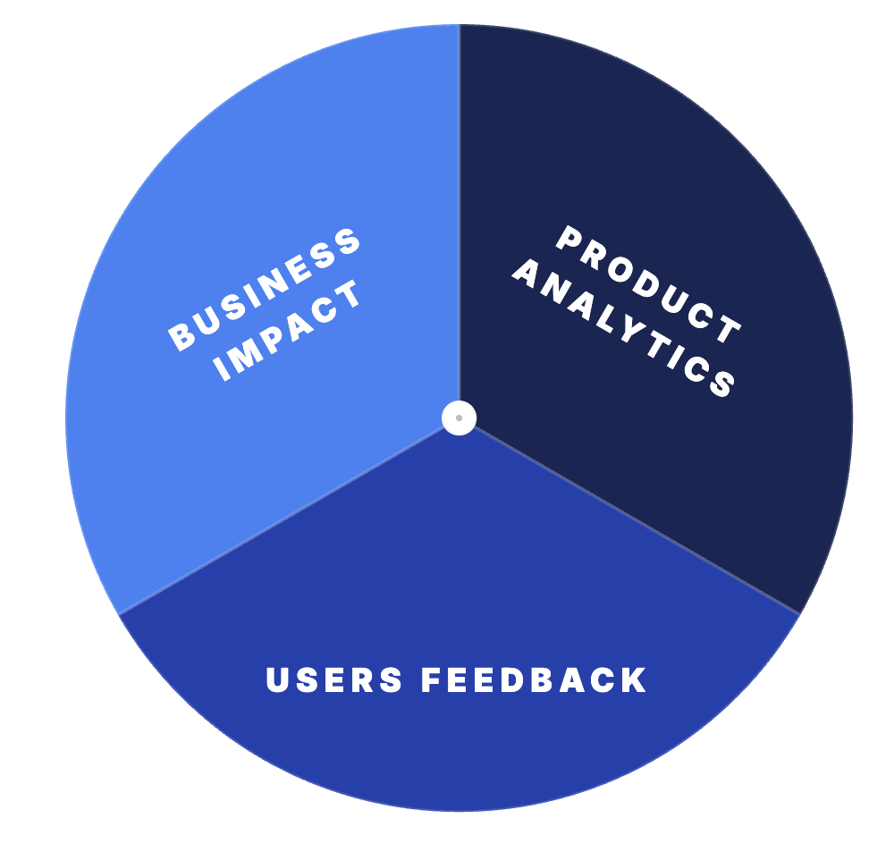
Validating selections: analytics + person suggestions + enterprise impression
A characteristic or change is a powerful match when you may verify the speculation from three angles:
Product analytics
Consumer suggestions
Enterprise impression
Consumer suggestions and analytics feeding product selections
If all three assist the identical determination, it’s a lot simpler to maneuver ahead. If they don’t, it normally means the speculation was not particular sufficient.
How we apply this at DevNet
Right here is how that loop – speculation, analytics, suggestions, determination – works in actual examples.
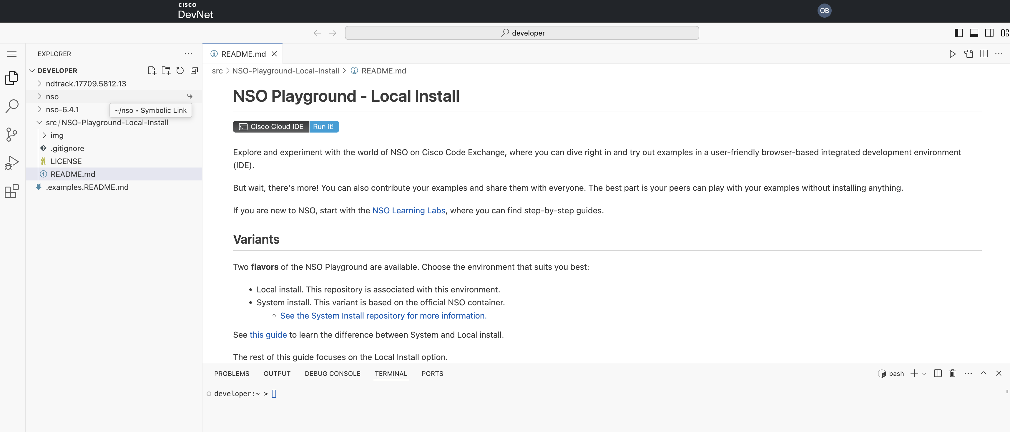
Instance 1: README-first Cloud IDE
Throughout common UX and suggestions classes, customers advised us they wished to see a repo’s README with directions and associated content material, and a clearer information on methods to use the IDE itself, whereas working with code samples within the Code Alternate Cloud IDE. A few of these environments are distinctive, corresponding to Cisco NSO containers that customers can spin up immediately within the Cloud IDE.
Analytics confirmed the identical downside: the default “Get began with VS Code” window was distracting customers relatively than serving to them.
We ran a comparative evaluation throughout two durations, complete pages analyzed, pages with classes below 2 minutes, the share of low-duration pages, complete views, the shortest session period, and the variety of important pages with a mean period below 15 seconds. The information confirmed the sample, and the answer was to open the repository README directions by default.
Up to date Cloud IDE interface with the repository README opened by default
Instance 2: Deprecating outdated repos with a related-repos widget
The second subject was a considerable amount of outdated code pattern content material. Wanting on the information, we noticed that these repositories nonetheless appeal to vital site visitors, so there was enterprise worth in dealing with them rigorously. There have been two choices:
Take away the pages fully and let customers hit a 404.
Deprecate them, present a transparent deprecation message, and show a widget with different associated repos.
We selected possibility 2 as a result of it provides customers a extra constant expertise and factors them to content material that also works.
Widget with associated repos on Code Alternate
Instance 3: “Developed by” filters within the MCP catalog
Just a few months in the past, we launched the AI repo catalog on Code Alternate, the place we collect MCP servers and AI brokers associated to Cisco applied sciences. In UX classes, customers advised us they wished to differentiate between MCP servers launched by product groups and people launched by the neighborhood:
Product-team MCP servers are usually a extra steady alternative, and most of them are distant.
Neighborhood MCP servers are open supply, so customers can learn the code and configure MCP instruments, prompts, or assets themselves.
Each varieties are beneficial, however customers wished to rapidly distinguish between them. To handle this, we added filtering choices and launched a devoted badge highlighting Cisco-developed servers.
“Developed by” filters on the MCP catalog
Be part of DevNet suggestions classes
Many of those modifications began in person expertise classes. Analytics can present us the place customers drop off or wrestle, however speaking to customers helps us perceive why and what to enhance subsequent.
Wish to share your suggestions about developer content material and the Cisco DevNet platform? Write to us at devnet_feedback@cisco.com.
On this submit we are going to study making time sequence predictions utilizing the sunspots dataset that ships with base R. Sunspots are darkish spots on the solar, related to decrease temperature. Right here’s a picture from NASA displaying the photo voltaic phenomenon.
We’re utilizing the month-to-month model of the dataset, sunspots.month (there’s a yearly model, too).
It comprises 265 years value of information (from 1749 by means of 2013) on the variety of sunspots monthly.
Forecasting this dataset is difficult due to excessive brief time period variability in addition to long-term irregularities evident within the cycles. For instance, most amplitudes reached by the low frequency cycle differ rather a lot, as does the variety of excessive frequency cycle steps wanted to achieve that most low frequency cycle top.
Our submit will deal with two dominant points: the way to apply deep studying to time sequence forecasting, and the way to correctly apply cross validation on this area.
For the latter, we are going to use the rsample bundle that enables to do resampling on time sequence knowledge.
As to the previous, our purpose is to not attain utmost efficiency however to point out the final plan of action when utilizing recurrent neural networks to mannequin this sort of knowledge.
Recurrent neural networks
When our knowledge has a sequential construction, it’s recurrent neural networks (RNNs) we use to mannequin it.
As of immediately, amongst RNNs, the perfect established architectures are the GRU (Gated Recurrent Unit) and the LSTM (Lengthy Brief Time period Reminiscence). For immediately, let’s not zoom in on what makes them particular, however on what they’ve in widespread with probably the most stripped-down RNN: the essential recurrence construction.
In distinction to the prototype of a neural community, typically referred to as Multilayer Perceptron (MLP), the RNN has a state that’s carried on over time. That is properly seen on this diagram from Goodfellow et al., a.okay.a. the “bible of deep studying”:
At every time, the state is a mixture of the present enter and the earlier hidden state. That is paying homage to autoregressive fashions, however with neural networks, there must be some level the place we halt the dependence.
That’s as a result of as a way to decide the weights, we maintain calculating how our loss modifications because the enter modifications.
Now if the enter now we have to contemplate, at an arbitrary timestep, ranges again indefinitely – then we will be unable to calculate all these gradients.
In apply, then, our hidden state will, at each iteration, be carried ahead by means of a set variety of steps.
We’ll come again to that as quickly as we’ve loaded and pre-processed the info.
Setup, pre-processing, and exploration
Libraries
Right here, first, are the libraries wanted for this tutorial.
When you’ve got not beforehand run Keras in R, you have to to put in Keras utilizing the install_keras() perform.
# Set up Keras you probably have not put in earlier thaninstall_keras()
Knowledge
sunspot.month is a ts class (not tidy), so we’ll convert to a tidy knowledge set utilizing the tk_tbl() perform from timetk. We use this as a substitute of as.tibble() from tibble to routinely protect the time sequence index as a zooyearmon index. Final, we’ll convert the zoo index to this point utilizing lubridate::as_date() (loaded with tidyquant) after which change to a tbl_time object to make time sequence operations simpler.
# A time tibble: 3,177 x 2
# Index: index
   index      worth

 1 1749-01-01  58
 2 1749-02-01  62.6
 3 1749-03-01  70
 4 1749-04-01  55.7
 5 1749-05-01  85
 6 1749-06-01  83.5
 7 1749-07-01  94.8
 8 1749-08-01  66.3
 9 1749-09-01  75.9
10 1749-10-01  75.5
# ... with 3,167 extra rows
Exploratory knowledge evaluation
The time sequence is lengthy (265 years!). We are able to visualize the time sequence each in full, and zoomed in on the primary 10 years to get a really feel for the sequence.
Visualizing sunspot knowledge with cowplot
We’ll make two ggplots and mix them utilizing cowplot::plot_grid(). Word that for the zoomed in plot, we make use of tibbletime::time_filter(), which is a straightforward option to carry out time-based filtering.
p1<-sun_spots%>%ggplot(aes(index, worth))+geom_point(coloration =palette_light()[[1]], alpha =0.5)+theme_tq()+labs( title ="From 1749 to 2013 (Full Knowledge Set)")p2<-sun_spots%>%filter_time("begin"~"1800")%>%ggplot(aes(index, worth))+geom_line(coloration =palette_light()[[1]], alpha =0.5)+geom_point(coloration =palette_light()[[1]])+geom_smooth(methodology ="loess", span =0.2, se =FALSE)+theme_tq()+labs( title ="1749 to 1759 (Zoomed In To Present Adjustments over the Yr)", caption ="datasets::sunspot.month")p_title<-ggdraw()+draw_label("Sunspots", dimension =18, fontface ="daring", color =palette_light()[[1]])plot_grid(p_title, p1, p2, ncol =1, rel_heights =c(0.1, 1, 1))
Backtesting: time sequence cross validation
When doing cross validation on sequential knowledge, the time dependencies on previous samples should be preserved. We are able to create a cross validation sampling plan by offsetting the window used to pick sequential sub-samples. In essence, we’re creatively coping with the truth that there’s no future take a look at knowledge accessible by creating a number of artificial “futures” – a course of typically, esp. in finance, referred to as “backtesting”.
As talked about within the introduction, the rsample bundle contains facitlities for backtesting on time sequence. The vignette, “Time Collection Evaluation Instance”, describes a process that makes use of the rolling_origin() perform to create samples designed for time sequence cross validation. We’ll use this method.
Creating a backtesting technique
The sampling plan we create makes use of 100 years (preliminary = 12 x 100 samples) for the coaching set and 50 years (assess = 12 x 50) for the testing (validation) set. We choose a skip span of about 22 years (skip = 12 x 22 – 1) to roughly evenly distribute the samples into 6 units that span your complete 265 years of sunspots historical past. Final, we choose cumulative = FALSE to permit the origin to shift which ensures that fashions on newer knowledge will not be given an unfair benefit (extra observations) over these working on much less latest knowledge. The tibble return comprises the rolling_origin_resamples.
# Rolling origin forecast resampling
# A tibble: 6 x 2
  splits       id

1  Slice1
2  Slice2
3  Slice3
4  Slice4
5  Slice5
6  Slice6
Visualizing the backtesting technique
We are able to visualize the resamples with two customized features. The primary, plot_split(), plots one of many resampling splits utilizing ggplot2. Word that an expand_y_axis argument is added to develop the date vary to the total sun_spots dataset date vary. This may grow to be helpful once we visualize all plots collectively.
# Plotting perform for a single break upplot_split<-perform(break up, expand_y_axis=TRUE, alpha=1, dimension=1, base_size=14){# Manipulate knowledgetrain_tbl<-coaching(break up)%>%add_column(key ="coaching")test_tbl<-testing(break up)%>%add_column(key ="testing")data_manipulated<-bind_rows(train_tbl, test_tbl)%>%as_tbl_time(index =index)%>%mutate(key =fct_relevel(key, "coaching", "testing"))# Gather attributestrain_time_summary<-train_tbl%>%tk_index()%>%tk_get_timeseries_summary()test_time_summary<-test_tbl%>%tk_index()%>%tk_get_timeseries_summary()# Visualizeg<-data_manipulated%>%ggplot(aes(x =index, y =worth, coloration =key))+geom_line(dimension =dimension, alpha =alpha)+theme_tq(base_size =base_size)+scale_color_tq()+labs( title =glue("Break up: {break up$id}"), subtitle =glue("{train_time_summary$begin} to ", "{test_time_summary$finish}"), y ="", x ="")+theme(legend.place ="none")if(expand_y_axis){sun_spots_time_summary<-sun_spots%>%tk_index()%>%tk_get_timeseries_summary()g<-g+scale_x_date(limits =c(sun_spots_time_summary$begin, sun_spots_time_summary$finish))}g}
The plot_split() perform takes one break up (on this case Slice01), and returns a visible of the sampling technique. We develop the axis to the vary for the total dataset utilizing expand_y_axis = TRUE.
The second perform, plot_sampling_plan(), scales the plot_split() perform to all the samples utilizing purrr and cowplot.
# Plotting perform that scales to all splits plot_sampling_plan<-perform(sampling_tbl, expand_y_axis=TRUE, ncol=3, alpha=1, dimension=1, base_size=14, title="Sampling Plan"){# Map plot_split() to sampling_tblsampling_tbl_with_plots<-sampling_tbl%>%mutate(gg_plots =map(splits, plot_split, expand_y_axis =expand_y_axis, alpha =alpha, base_size =base_size))# Make plots with cowplotplot_list<-sampling_tbl_with_plots$gg_plotsp_temp<-plot_list[[1]]+theme(legend.place ="backside")legend<-get_legend(p_temp)p_body<-plot_grid(plotlist =plot_list, ncol =ncol)p_title<-ggdraw()+draw_label(title, dimension =14, fontface ="daring", color =palette_light()[[1]])g<-plot_grid(p_title, p_body, legend, ncol =1, rel_heights =c(0.05, 1, 0.05))g}
We are able to now visualize your complete backtesting technique with plot_sampling_plan(). We are able to see how the sampling plan shifts the sampling window with every progressive slice of the practice/take a look at splits.
rolling_origin_resamples%>%plot_sampling_plan(expand_y_axis =T, ncol =3, alpha =1, dimension =1, base_size =10, title ="Backtesting Technique: Rolling Origin Sampling Plan")
And, we will set expand_y_axis = FALSE to zoom in on the samples.
We’ll use this backtesting technique (6 samples from one time sequence every with 50/10 break up in years and a ~20 12 months offset) when testing the veracity of the LSTM mannequin on the sunspots dataset.
The LSTM mannequin
To start, we’ll develop an LSTM mannequin on a single pattern from the backtesting technique, particularly, the latest slice. We’ll then apply the mannequin to all samples to research modeling efficiency.
To help hyperparameter tuning, apart from the coaching set we additionally want a validation set.
For instance, we are going to use a callback, callback_early_stopping, that stops coaching when no vital efficiency is seen on the validation set (what’s thought-about vital is as much as you).
We’ll dedicate 2 thirds of the evaluation set to coaching, and 1 third to validation.
df_trn<-evaluation(example_split)[1:800, , drop =FALSE]df_val<-evaluation(example_split)[801:1200, , drop =FALSE]df_tst<-evaluation(example_split)
First, let’s mix the coaching and testing knowledge units right into a single knowledge set with a column key that specifies the place they got here from (both “coaching” or “testing)”. Word that the tbl_time object might want to have the index respecified through the bind_rows() step, however this challenge must be corrected in dplyr quickly.
# A time tibble: 1,800 x 3
# Index: index
   index      worth key

 1 1849-06-01  81.1 coaching
 2 1849-07-01  78   coaching
 3 1849-08-01  67.7 coaching
 4 1849-09-01  93.7 coaching
 5 1849-10-01  71.5 coaching
 6 1849-11-01  99   coaching
 7 1849-12-01  97   coaching
 8 1850-01-01  78   coaching
 9 1850-02-01  89.4 coaching
10 1850-03-01  82.6 coaching
# ... with 1,790 extra rows
Preprocessing with recipes
The LSTM algorithm will normally work higher if the enter knowledge has been centered and scaled. We are able to conveniently accomplish this utilizing the recipes bundle. Along with step_center and step_scale, we’re utilizing step_sqrt to cut back variance and remov outliers. The precise transformations are executed once we bake the info in accordance with the recipe:
Subsequent, let’s seize the unique heart and scale so we will invert the steps after modeling. The sq. root step can then merely be undone by squaring the back-transformed knowledge.
Keras LSTM expects the enter in addition to the goal knowledge to be in a particular form.
The enter must be a 3D array of dimension num_samples, num_timesteps, num_features.
Right here, num_samples is the variety of observations within the set. This may get fed to the mannequin in parts of batch_size. The second dimension, num_timesteps, is the size of the hidden state we have been speaking about above. Lastly, the third dimension is the variety of predictors we’re utilizing. For univariate time sequence, that is 1.
How lengthy ought to we select the hidden state to be? This typically is determined by the dataset and our purpose.
If we did one-step-ahead forecasts – thus, forecasting the next month solely – our important concern can be selecting a state size that enables to study any patterns current within the knowledge.
Now say we wished to forecast 12 months as a substitute, as does SILSO, the World Knowledge Heart for the manufacturing, preservation and dissemination of the worldwide sunspot quantity.
The way in which we will do that, with Keras, is by wiring the LSTM hidden states to units of consecutive outputs of the identical size. Thus, if we wish to produce predictions for 12 months, our LSTM ought to have a hidden state size of 12.
These 12 time steps will then get wired to 12 linear predictor items utilizing a time_distributed() wrapper.
That wrapper’s process is to use the identical calculation (i.e., the identical weight matrix) to each state enter it receives.
Now, what’s the goal array’s format presupposed to be? As we’re forecasting a number of timesteps right here, the goal knowledge once more must be three-d. Dimension 1 once more is the batch dimension, dimension 2 once more corresponds to the variety of timesteps (the forecasted ones), and dimension 3 is the dimensions of the wrapped layer.
In our case, the wrapped layer is a layer_dense() of a single unit, as we wish precisely one prediction per time limit.
So, let’s reshape the info. The principle motion right here is creating the sliding home windows of 12 steps of enter, adopted by 12 steps of output every. That is best to grasp with a shorter and less complicated instance. Say our enter have been the numbers from 1 to 10, and our chosen sequence size (state dimension) have been 4. Tthis is how we’d need our coaching enter to look:
1,2,3,4
2,3,4,5
3,4,5,6
And our goal knowledge, correspondingly:
5,6,7,8
6,7,8,9
7,8,9,10
We’ll outline a brief perform that does this reshaping on a given dataset.
Then lastly, we add the third axis that’s formally wanted (regardless that that axis is of dimension 1 in our case).
# these variables are being outlined simply due to the order through which# we current issues on this submit (first the info, then the mannequin)# they are going to be outdated by FLAGS$n_timesteps, FLAGS$batch_size and n_predictions# within the following snippetn_timesteps<-12n_predictions<-n_timestepsbatch_size<-10# features usedbuild_matrix<-perform(tseries, overall_timesteps){t(sapply(1:(size(tseries)-overall_timesteps+1), perform(x)tseries[x:(x+overall_timesteps-1)]))}reshape_X_3d<-perform(X){dim(X)<-c(dim(X)[1], dim(X)[2], 1)X}# extract values from knowledge bodytrain_vals<-df_processed_tbl%>%filter(key=="coaching")%>%choose(worth)%>%pull()valid_vals<-df_processed_tbl%>%filter(key=="validation")%>%choose(worth)%>%pull()test_vals<-df_processed_tbl%>%filter(key=="testing")%>%choose(worth)%>%pull()# construct the windowed matricestrain_matrix<-build_matrix(train_vals, n_timesteps+n_predictions)valid_matrix<-build_matrix(valid_vals, n_timesteps+n_predictions)test_matrix<-build_matrix(test_vals, n_timesteps+n_predictions)# separate matrices into coaching and testing components# additionally, discard final batch if there are fewer than batch_size samples# (a purely technical requirement)X_train<-train_matrix[, 1:n_timesteps]y_train<-train_matrix[, (n_timesteps+1):(n_timesteps*2)]X_train<-X_train[1:(nrow(X_train)%/%batch_size*batch_size), ]y_train<-y_train[1:(nrow(y_train)%/%batch_size*batch_size), ]X_valid<-valid_matrix[, 1:n_timesteps]y_valid<-valid_matrix[, (n_timesteps+1):(n_timesteps*2)]X_valid<-X_valid[1:(nrow(X_valid)%/%batch_size*batch_size), ]y_valid<-y_valid[1:(nrow(y_valid)%/%batch_size*batch_size), ]X_test<-test_matrix[, 1:n_timesteps]y_test<-test_matrix[, (n_timesteps+1):(n_timesteps*2)]X_test<-X_test[1:(nrow(X_test)%/%batch_size*batch_size), ]y_test<-y_test[1:(nrow(y_test)%/%batch_size*batch_size), ]# add on the required third axisX_train<-reshape_X_3d(X_train)X_valid<-reshape_X_3d(X_valid)X_test<-reshape_X_3d(X_test)y_train<-reshape_X_3d(y_train)y_valid<-reshape_X_3d(y_valid)y_test<-reshape_X_3d(y_test)
Constructing the LSTM mannequin
Now that now we have our knowledge within the required kind, let’s lastly construct the mannequin.
As at all times in deep studying, an essential, and sometimes time-consuming, a part of the job is tuning hyperparameters. To maintain this submit self-contained, and contemplating that is primarily a tutorial on the way to use LSTM in R, let’s assume the next settings have been discovered after in depth experimentation (in actuality experimentation did happen, however to not a level that efficiency couldn’t presumably be improved).
As an alternative of exhausting coding the hyperparameters, we’ll use tfruns to arrange an setting the place we might simply carry out grid search.
We’ll rapidly touch upon what these parameters do however primarily depart these subjects to additional posts.
FLAGS<-flags(# There's a so-called "stateful LSTM" in Keras. Whereas LSTM is stateful# per se, this provides an additional tweak the place the hidden states get # initialized with values from the merchandise at similar place within the earlier# batch. That is useful slightly below particular circumstances, or if you need# to create an "infinite stream" of states, through which case you'd use 1 as # the batch dimension. Under, we present how the code must be modified to# use this, nevertheless it will not be additional mentioned right here.flag_boolean("stateful", FALSE),# Ought to we use a number of layers of LSTM?# Once more, simply included for completeness, it didn't yield any superior # efficiency on this process.# This may truly stack precisely one extra layer of LSTM items.flag_boolean("stack_layers", FALSE),# variety of samples fed to the mannequin in a single goflag_integer("batch_size", 10),# dimension of the hidden state, equals dimension of predictionsflag_integer("n_timesteps", 12),# what number of epochs to coach forflag_integer("n_epochs", 100),# fraction of the items to drop for the linear transformation of the inputsflag_numeric("dropout", 0.2),# fraction of the items to drop for the linear transformation of the # recurrent stateflag_numeric("recurrent_dropout", 0.2),# loss perform. Discovered to work higher for this particular case than imply# squared errorflag_string("loss", "logcosh"),# optimizer = stochastic gradient descent. Appeared to work higher than adam # or rmsprop right here (as indicated by restricted testing)flag_string("optimizer_type", "sgd"),# dimension of the LSTM layerflag_integer("n_units", 128),# studying feeflag_numeric("lr", 0.003),# momentum, a further parameter to the SGD optimizerflag_numeric("momentum", 0.9),# parameter to the early stopping callbackflag_integer("endurance", 10))# the variety of predictions we'll make equals the size of the hidden staten_predictions<-FLAGS$n_timesteps# what number of options = predictors now we haven_features<-1# simply in case we wished to attempt totally different optimizers, we might add right hereoptimizer<-change(FLAGS$optimizer_type, sgd =optimizer_sgd(lr =FLAGS$lr, momentum =FLAGS$momentum))# callbacks to be handed to the match() perform# We simply use one right here: we might cease earlier than n_epochs if the loss on the# validation set doesn't lower (by a configurable quantity, over a # configurable time)callbacks<-checklist(callback_early_stopping(endurance =FLAGS$endurance))
In spite of everything these preparations, the code for developing and coaching the mannequin is slightly brief!
Let’s first rapidly view the “lengthy model”, that may will let you take a look at stacking a number of LSTMs or use a stateful LSTM, then undergo the ultimate brief model (that does neither) and touch upon it.
Now let’s step by means of the less complicated, but higher (or equally) performing configuration under.
# create the mannequinmannequin<-keras_model_sequential()# add layers# now we have simply two, the LSTM and the time_distributed mannequin%>%layer_lstm( items =FLAGS$n_units, # the primary layer in a mannequin must know the form of the enter knowledge batch_input_shape =c(FLAGS$batch_size, FLAGS$n_timesteps, n_features), dropout =FLAGS$dropout, recurrent_dropout =FLAGS$recurrent_dropout,# by default, an LSTM simply returns the ultimate state return_sequences =TRUE)%>%time_distributed(layer_dense(items =1))mannequin%>%compile( loss =FLAGS$loss, optimizer =optimizer,# along with the loss, Keras will inform us about present # MSE whereas coaching metrics =checklist("mean_squared_error"))historical past<-mannequin%>%match( x =X_train, y =y_train, validation_data =checklist(X_valid, y_valid), batch_size =FLAGS$batch_size, epochs =FLAGS$n_epochs, callbacks =callbacks)
As we see, coaching was stopped after ~55 epochs as validation loss didn’t lower any extra.
We additionally see that efficiency on the validation set is approach worse than efficiency on the coaching set – usually indicating overfitting.
This matter too, we’ll depart to a separate dialogue one other time, however apparently regularization utilizing larger values of dropout and recurrent_dropout (mixed with growing mannequin capability) didn’t yield higher generalization efficiency. That is in all probability associated to the traits of this particular time sequence we talked about within the introduction.
Now let’s see how nicely the mannequin was in a position to seize the traits of the coaching set.
pred_train<-mannequin%>%predict(X_train, batch_size =FLAGS$batch_size)%>%.[, , 1]# Retransform values to unique scalepred_train<-(pred_train*scale_history+center_history)^2compare_train<-df%>%filter(key=="coaching")# construct a dataframe that has each precise and predicted valuesfor(iin1:nrow(pred_train)){varname<-paste0("pred_train", i)compare_train<-mutate(compare_train,!!varname:=c(rep(NA, FLAGS$n_timesteps+i-1),pred_train[i,],rep(NA, nrow(compare_train)-FLAGS$n_timesteps*2-i+1)))}
We compute the typical RSME over all sequences of predictions.
How do these predictions actually look? As a visualization of all predicted sequences would look fairly crowded, we arbitrarily choose begin factors at common intervals.
This seems fairly good. From the validation loss, we don’t fairly count on the identical from the take a look at set, although.
Let’s see.
pred_test<-mannequin%>%predict(X_test, batch_size =FLAGS$batch_size)%>%.[, , 1]# Retransform values to unique scalepred_test<-(pred_test*scale_history+center_history)^2pred_test[1:10, 1:5]%>%print()compare_test<-df%>%filter(key=="testing")# construct a dataframe that has each precise and predicted valuesfor(iin1:nrow(pred_test)){varname<-paste0("pred_test", i)compare_test<-mutate(compare_test,!!varname:=c(rep(NA, FLAGS$n_timesteps+i-1),pred_test[i,],rep(NA, nrow(compare_test)-FLAGS$n_timesteps*2-i+1)))}compare_test%>%write_csv(str_replace(model_path, ".hdf5", ".take a look at.csv"))compare_test[FLAGS$n_timesteps:(FLAGS$n_timesteps+10), c(2, 4:8)]%>%print()coln<-colnames(compare_test)[4:ncol(compare_test)]cols<-map(coln, quo(sym(.)))rsme_test<-map_dbl(cols, perform(col)rmse(compare_test, reality =worth, estimate =!!col, na.rm =TRUE))%>%imply()rsme_test
31.31616
ggplot(compare_test, aes(x =index, y =worth))+geom_line()+geom_line(aes(y =pred_test1), coloration ="cyan")+geom_line(aes(y =pred_test50), coloration ="purple")+geom_line(aes(y =pred_test100), coloration ="inexperienced")+geom_line(aes(y =pred_test150), coloration ="violet")+geom_line(aes(y =pred_test200), coloration ="cyan")+geom_line(aes(y =pred_test250), coloration ="purple")+geom_line(aes(y =pred_test300), coloration ="inexperienced")+geom_line(aes(y =pred_test350), coloration ="cyan")+geom_line(aes(y =pred_test400), coloration ="purple")+geom_line(aes(y =pred_test450), coloration ="inexperienced")+geom_line(aes(y =pred_test500), coloration ="cyan")+geom_line(aes(y =pred_test550), coloration ="violet")+ggtitle("Predictions on take a look at set")
That’s not so good as on the coaching set, however not dangerous both, given this time sequence is sort of difficult.
Having outlined and run our mannequin on a manually chosen instance break up, let’s now revert to our general re-sampling body.
Backtesting the mannequin on all splits
To acquire predictions on all splits, we transfer the above code right into a perform and apply it to all splits.
First, right here’s the perform. It returns a listing of two dataframes, one for the coaching and take a look at units every, that comprise the mannequin’s predictions along with the precise values.
How does it look? Right here’s RMSE on the coaching set for the 6 splits.
# A tibble: 6 x 2
  id      rmse

1 Slice1  22.2
2 Slice2  20.9
3 Slice3  18.8
4 Slice4  23.5
5 Slice5  22.1
6 Slice6  21.1
# A tibble: 6 x 2
  id      rmse

1 Slice1  21.6
2 Slice2  20.6
3 Slice3  21.3
4 Slice4  31.4
5 Slice5  35.2
6 Slice6  31.4
Taking a look at these numbers, we see one thing attention-grabbing: Generalization efficiency is a lot better for the primary three slices of the time sequence than for the latter ones. This confirms our impression, said above, that there appears to be some hidden improvement happening, rendering forecasting tougher.
And listed below are visualizations of the predictions on the respective coaching and take a look at units.
This has been an extended submit, and essentially can have left numerous questions open, at the start: How will we acquire good settings for the hyperparameters (studying fee, variety of epochs, dropout)?
How will we select the size of the hidden state? And even, can now we have an instinct how nicely LSTM will carry out on a given dataset (with its particular traits)?
We’ll sort out questions just like the above in upcoming posts.
There’s all the time that second when it is advisable scan one thing — a receipt, a kind, a contract — and all of a sudden you’re caught with out a printer, a scanner, or the endurance to take care of both. Taking a photograph works… till it doesn’t. That’s the place one thing extra purpose-built begins to make sense. This iScanner App lifetime subscription is right down to $25.97 (MSRP $199.90), turning your telephone right into a full-on doc hub.
As an alternative of snapping messy images, iScanner robotically detects edges, straightens pages, and cleans up the picture so your scans truly appear to be correct paperwork. It will probably export recordsdata in a number of codecs like PDF, Phrase, or JPG, and even pulls textual content from scans utilizing OCR so you may edit or search them later. The app additionally doubles as a light-weight editor and file supervisor, so you may signal paperwork, manage recordsdata, and hold the whole lot in a single place.
iScanner turns your telephone into the final word doc hub
Scan paperwork, IDs, receipts, and notes in seconds
Convert recordsdata to PDF, Phrase, Excel, and extra
Within the remoted forests encroaching on the ruins of the Chernobyl exclusion zone, too harmful for people to inhabit, wolves are mysteriously thriving.
Within the 40 years for the reason that 26 April 1986 catastrophic explosion of the Chernobyl Nuclear Energy Plant’s Unit 4 reactor close to the city of Pripyat, Ukraine, massive numbers of animals have moved in to benefit from a habitat freed from people.
Amongst these are the grey wolves (Canis lupus), prime predators whose inhabitants density within the exclusion zone has boomed since 1986.
Now, a brand new genetic examine may be serving to scientists perceive why.
The wolves, in response to researchers led by evolutionary biologists Cara Love and Shane Campbell-Staton of Princeton College, have genetic variations from wolves in different components of the world that recommend they could be creating traits that assist them address the area’s pervasive ionizing radiation.
“There could also be genetic variation inside the inhabitants which will enable some people to be extra resistant or resilient within the face of that radiation, through which case they could nonetheless get most cancers on the identical fee, however it might not impression their operate as a lot as it might, , a person exterior of the exclusion zone,” Campbell-Staton instructed NPR Quick Wave in 2024.
What we nonetheless do not actually know is how that attainable resistance or resilience works.
“They’re simply capable of take that burden higher for some cause. Or it might be resistance,” Campbell-Staton stated, “and regardless of that stress – that radiation publicity – they only do not get most cancers as a lot.”
Within the a long time for the reason that nuclear catastrophe, people within the area have been scarce.
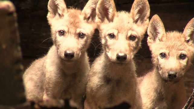
Wolf cubs in an deserted village within the Chernobyl exclusion zone. (Movie Studio Aves/Creatas Video/Getty Photos)
This appears to have created a form of radioactive Backyard of Eden.
Animals in droves have taken over the 4,200 sq. kilometers (1,620 sq. miles) coated by the reserves, together with wild animals reminiscent of deer, bison, boar, and wolves, in addition to packs of canines descended from the pets left behind by the numerous hundreds of evacuees from the cities and villages.
Nevertheless, in response to a 2015 census of animal populations within the zone, one inhabitants actually stands out.
“Relative abundances of elk, roe deer, pink deer, and wild boar inside the Chernobyl exclusion zone are just like these in 4 (uncontaminated) nature reserves within the area,” writes a crew led by wildlife ecologist Tatiana Deryabina of the Polesie State Radioecological Reserve.
“Wolf abundance is greater than seven instances larger.”
The work of Love, Campbell-Staton, and their colleagues sought to reply the query of why wolf populations had ballooned whereas different animal populations remained comparatively constant.
In 2024, they entered the exclusion zone and picked up blood samples from a number of wolves. Additionally they took blood samples from wolves in Belarus, the place radiation ranges are decrease, and from wolves in Yellowstone Nationwide Park within the US, the place ionizing radiation is at Earth’s regular baseline.
They discovered 3,180 genes that behave otherwise within the Chernobyl wolves in comparison with the opposite populations.
Subsequent, they in contrast this genetic dataset with human genetic information from The Most cancers Genome Atlas (TCGA), searching for markers of 10 kinds of tumors that people and canines share.
Crucially, they discovered 23 cancer-related genes which are extra lively in Chernobyl wolves – and these genes are related to higher survival charges for some cancers in people. The fastest-evolving areas had been in and round genes related to anti-cancer and anti-tumor responses in mammals.
The genetic profile of the Chernobyl wolves is probably going formed by extended radiation publicity over many generations, the researchers stated. These animals reside in a radioactive space, consuming radiation-exposed herbivores that eat radiation-exposed vegetation, all of which accumulate over time.
“Grey wolves provide a extremely attention-grabbing alternative to grasp the impacts of continual, low-dose, multigenerational publicity to ionizing radiation due to the function that they play of their ecosystems,” Campbell-Staton stated.
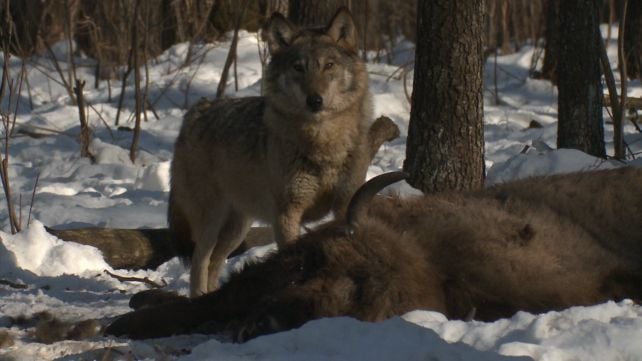
Wolves within the zone prey on different animals, reminiscent of bison and deer. (Movie Studio Aves/Creatas Video/Getty Photos)
It is not clear precisely how this genetic profile works in observe. The wolves might get much less most cancers, or they could have higher most cancers survival charges, or a mix of each.
The researchers have ready a paper describing their findings, first detailed in a convention presentation in 2024. The hope is that, in addition to yielding insights into animal resilience, this may occasionally even be related to human most cancers analysis.
“We’ve began collaborating with most cancers biologists and most cancers firms to assist us to interpret these information after which attempt to determine if there are any straight translatable variations which will provide, like, novel therapeutic targets for most cancers in people, as an illustration,” Campbell-Staton stated.
Editor’s be aware: This text makes use of the spelling “Chernobyl” to replicate the historic context of the 1986 catastrophe, when Ukraine was a part of the Soviet Union and Russian transliterations had been extensively used. The Ukrainian spelling is “Chornobyl”.


