Friday, February 13, 2026
Home Blog Page 37

Revolutionizing Healthcare with Multimodal AI: The Subsequent Frontier


How can healthcare selections grow to be extra correct when affected person knowledge is scattered throughout reviews, photos, and monitoring techniques? 

Regardless of advances in synthetic intelligence, most healthcare AI instruments nonetheless function in silos, limiting their real-world impression, and that is the place the Multimodal AI addresses this hole by integrating a number of knowledge varieties, corresponding to scientific textual content, medical imaging, and physiological indicators right into a unified intelligence framework.

On this weblog, we discover how multimodal AI is reworking healthcare by enabling extra context-aware diagnostics, personalised remedy methods, and environment friendly scientific workflows, whereas additionally highlighting why it represents the subsequent frontier for healthcare.

Summarize this text with ChatGPT
Get key takeaways & ask questions

What’s Multimodal AI?

Multimodal AI refers to synthetic intelligence techniques designed to course of and combine a number of kinds of knowledge concurrently. Multimodal AI can interpret mixtures of knowledge varieties to extract richer, extra contextual insights. 

In healthcare, this implies analyzing scientific notes, medical photos, lab outcomes, biosignals from wearables, and even patient-reported signs collectively reasonably than in isolation. 

By doing so, multimodal AI permits a extra correct understanding of affected person well being, bridging gaps that single-modality AI techniques usually go away unaddressed.

Core Modalities in Healthcare

  • Scientific Textual content: This consists of Digital Well being Data (EHRs), structured doctor notes, discharge summaries, and affected person histories. It supplies the “narrative” and context of a affected person’s journey.
  • Medical Imaging: Information from X-rays, MRIs, CT scans, and ultrasounds. AI can detect patterns in pixels that could be invisible to the human eye, corresponding to minute textural adjustments in tissue.
  • Biosignals: Steady knowledge streams from ECGs (coronary heart), EEGs (mind), and real-time vitals from hospital displays or shopper wearables (like smartwatches).
  • Audio: Pure language processing (NLP) utilized to doctor-patient conversations. This may seize nuances in speech, cough patterns for respiratory analysis, or cognitive markers in vocal tone.
  • Genomic and Lab Information: Massive-scale “Omics” knowledge (genomics, proteomics) and normal blood panels. These present the molecular-level floor reality of a affected person’s organic state.

How Multimodal Fusion Permits Holistic Affected person Understanding?

Multimodal fusion is the method of mixing and aligning knowledge from completely different modalities right into a unified illustration for AI fashions. This integration permits AI to:

  • Seize Interdependencies: Delicate patterns in imaging could correlate with lab anomalies or textual observations in affected person information.
  • Scale back Diagnostic Blind Spots: By cross-referencing a number of knowledge sources, clinicians can detect circumstances earlier and with greater confidence.
  • Help Customized Remedy: Multimodal fusion permits AI to grasp the affected person’s well being story in its entirety, together with medical historical past, genetics, way of life, and real-time vitals, enabling actually personalised interventions.
  • Improve Predictive Insights: Combining predictive modalities improves the AI’s capacity to forecast illness development, remedy response, and potential issues.

Instance:
In oncology, fusing MRI scans, biopsy outcomes, genetic markers, and scientific notes permits AI to advocate focused therapies tailor-made to the affected person’s distinctive profile, reasonably than counting on generalized remedy protocols.

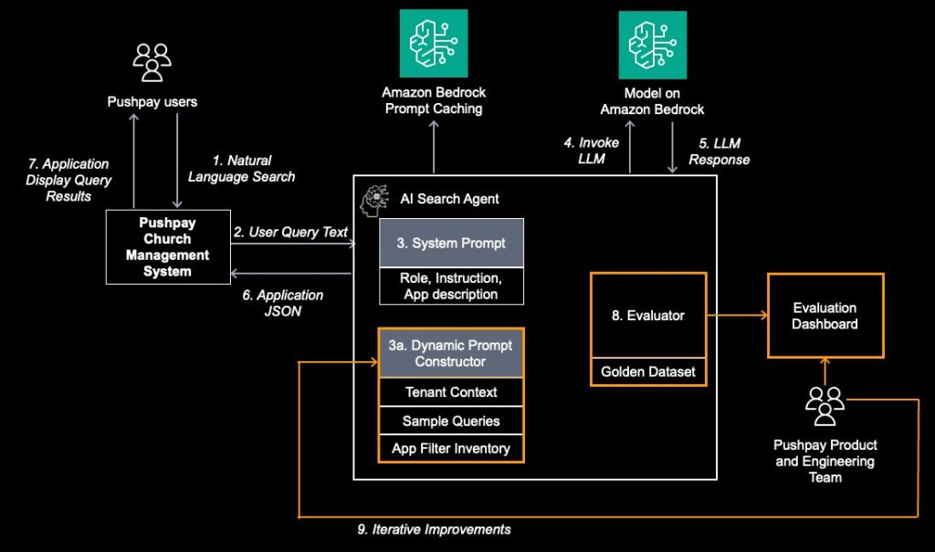
Structure Behind Multimodal Healthcare AI Techniques

Architecture Behind Multimodal Healthcare AI Systems

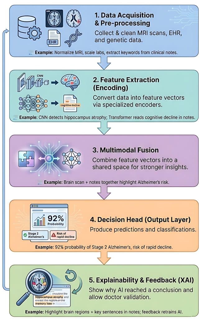
Constructing a multimodal healthcare AI system entails integrating various knowledge varieties, corresponding to medical photos, digital well being information (EHRs), and genomic sequences, to supply a complete view of a affected person’s well being. 

For instance this, let’s use the instance of diagnosing and predicting the development of Alzheimer’s Illness.

1. Information Acquisition and Pre-processing

On this stage, the system collects uncooked knowledge from numerous sources. As a result of these sources converse “completely different languages,” they have to be cleaned and standardized.

  • Imaging Information (Pc Imaginative and prescient): Uncooked MRI or PET scans are normalized for depth and resized.
  • Structured Information (Tabular): Affected person age, genetic markers (like APOE4 standing), and lab outcomes are scaled.
  • Unstructured Information (NLP): Scientific notes from neurologists are processed to extract key phrases like “reminiscence loss” or “disorientation.”

Every knowledge sort is shipped by means of a specialised encoder (a neural community) that interprets uncooked knowledge right into a mathematical illustration known as a function vector. Instance:

  • The CNN encoder processes the MRI and detects “atrophy within the hippocampus.”
  • The Transformer encoder processes scientific notes and identifies “progressive cognitive decline.”
  • The MLP encoder processes the genetic knowledge, flagging a excessive danger because of particular biomarkers.

3. Multimodal Fusion

That is the “mind” of the structure. The system should determine how you can mix these completely different function vectors. There are three frequent methods:

  • Early Fusion: Combining uncooked options instantly (usually messy because of completely different scales).
  • Late Fusion: Every mannequin makes a separate “vote,” and the outcomes are averaged.
  • Intermediate (Joint) Fusion: The commonest strategy, the place function vectors are projected right into a shared mathematical area to seek out correlations.
  • Instance: The system notices that the hippocampal shrinkage (from the picture) aligns completely with the low cognitive scores (from the notes), making a a lot stronger “sign” for Alzheimer’s than both would alone.

4. The Resolution Head (Output Layer)

The fused data is handed to a remaining set of absolutely related layers that produce the precise scientific output wanted. The Instance: The system outputs two issues:

  • Classification: “92% likelihood of Stage 2 Alzheimer’s.”
  • Prediction: “Excessive danger of speedy decline inside 12 months.”

5. Explainability and Suggestions Loop (XAI)

In healthcare, a “black field” is not sufficient. The system makes use of an explainability layer (like SHAP or Consideration Maps) to indicate the physician why it reached a conclusion. Instance: 

The system highlights the precise space of the mind scan and the precise sentences within the scientific notes that led to the analysis. The physician can then verify or right the output, which helps retrain the mannequin.

As multimodal AI turns into central to fashionable healthcare, there’s a rising want for professionals who can mix scientific information with technical experience.

The Johns Hopkins College’s AI in Healthcare Certificates Program equips you with expertise in medical imaging, precision medication, and regulatory frameworks like FDA and HIPAA, making ready you to design, consider, and implement secure, efficient AI techniques. Enroll at present to grow to be a future-ready healthcare AI skilled and drive the subsequent era of scientific innovation.

Excessive-Affect Use Circumstances Displaying Why Multimodal AI is The Subsequent Frontier in Healthcare

High-Impact Multimodal AI Use CasesHigh-Impact Multimodal AI Use Cases

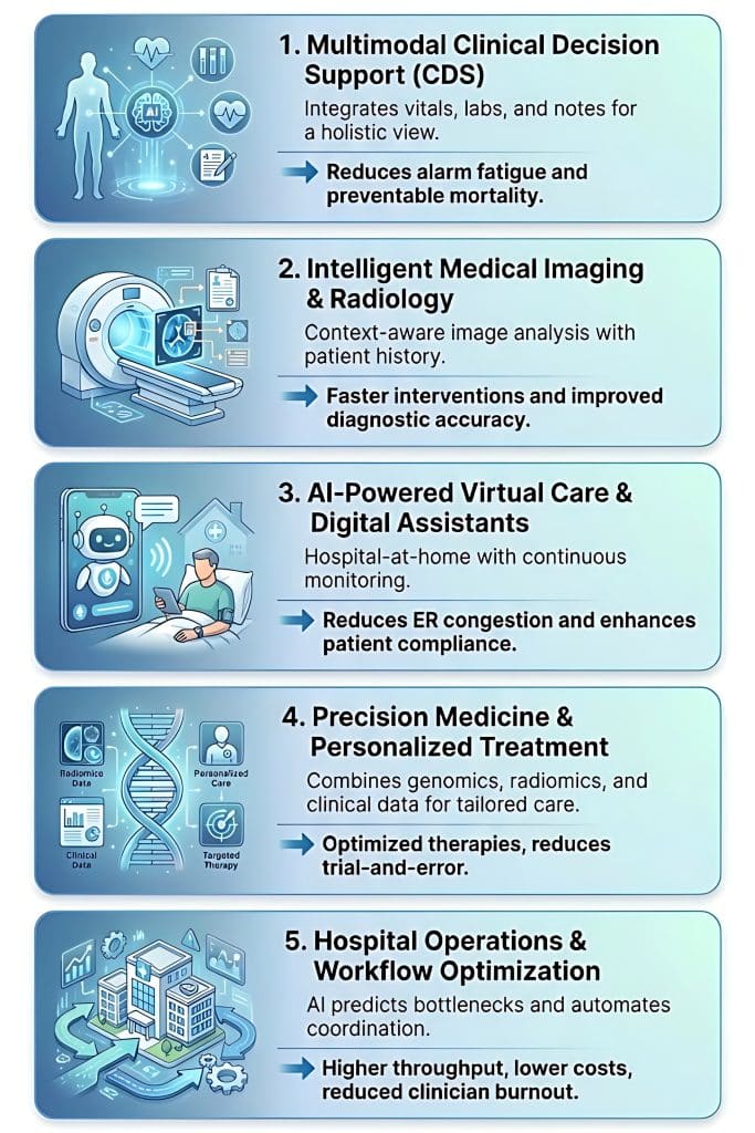
1. Multimodal Scientific Resolution Help (CDS)

Conventional scientific choice help (CDS) usually depends on remoted alerts, corresponding to a excessive coronary heart price set off. Multimodal CDS, nonetheless, integrates a number of streams of affected person data to supply a holistic view.

  • Integration: It correlates real-time important indicators, longitudinal laboratory outcomes, and unstructured doctor notes to create a complete affected person profile.
  • Early Detection: In circumstances like sepsis, AI can determine delicate adjustments in cognitive state or speech patterns from nurse notes hours earlier than important indicators deteriorate. In oncology, it combines pathology photos with genetic markers to detect aggressive mutations early.
  • Lowering Uncertainty: The system identifies and highlights conflicting knowledge, for instance, when lab outcomes recommend one analysis however bodily exams point out one other, enabling well timed human assessment.
  • Final result: This strategy reduces clinician “alarm fatigue” and helps 24/7 proactive monitoring, contributing to a measurable lower in preventable mortality.

2. Clever Medical Imaging & Radiology

Medical imaging is evolving from easy detection (“What’s on this picture?”) to patient-specific interpretation (“What does this picture imply for this affected person?”).

  • Context-Pushed Interpretation: AI cross-references imaging findings with scientific knowledge, corresponding to affected person historical past, prior biopsies, and documented signs, to supply significant insights.
  • Automated Prioritization: Scans are analyzed in real-time. For pressing findings, corresponding to intracranial hemorrhage, the system prioritizes these circumstances for instant radiologist assessment.
  • Augmentation: AI acts as a further professional, highlighting delicate abnormalities, offering automated measurements, and evaluating present scans with earlier imaging to help radiologists in decision-making.
  • Final result: This results in sooner emergency interventions and improved diagnostic accuracy, notably in complicated or uncommon circumstances, enhancing general affected person care.

3. AI-Powered Digital Care & Digital Assistants

AI-driven digital care instruments lengthen the attain of clinics into sufferers’ properties, enabling a “hospital at house” mannequin.

  • Holistic Triage: Digital assistants analyze a number of inputs, voice patterns, symptom descriptions, and wearable system knowledge to find out whether or not a affected person requires an emergency go to or will be managed at house.
  • Scientific Reminiscence: Not like fundamental chatbots, these techniques retain detailed affected person histories. As an illustration, a headache reported by a hypertension affected person is flagged with greater urgency than the identical symptom in a wholesome particular person.
  • Steady Engagement: Publish-surgery follow-ups are automated, guaranteeing medicine adherence, monitoring bodily remedy, and detecting potential issues corresponding to an contaminated surgical website earlier than hospital readmission turns into crucial.
  • Final result: This strategy reduces emergency division congestion, enhances affected person compliance, and improves satisfaction by means of personalised, steady care.

4. Precision Medication & Customized Remedy

Precision medication shifts healthcare from a “one-size-fits-all” strategy to therapies tailor-made to every affected person’s molecular and scientific profile.

  • Omics Integration: AI combines genomics, transcriptomics, and radiomics to assemble a complete, multi-dimensional map of a affected person’s illness.
  • Dosage Optimization: Utilizing real-time knowledge on kidney operate and genetic metabolism, AI predicts the exact chemotherapy dosage that maximizes effectiveness whereas minimizing toxicity.
  • Predictive Modeling: Digital twin simulations enable clinicians to forecast how a selected affected person will reply to completely different therapies, corresponding to immunotherapy versus chemotherapy, earlier than remedy begins.
  • Final result: This technique transforms beforehand terminal sicknesses into manageable circumstances and eliminates the normal trial-and-error strategy in high-risk therapies.

5. Hospital Operations & Workflow Optimization

AI applies multimodal analytics to the complicated, dynamic setting of hospital operations, treating the power as a “dwelling organism.”

  • Capability Planning: By analyzing components corresponding to seasonal sickness patterns, native occasions, staffing ranges, and affected person acuity within the ER, AI can precisely forecast mattress demand and put together assets prematurely.
  • Predicting Bottlenecks: The system identifies potential delays, for instance, a hold-up within the MRI suite that would cascade into surgical discharge delay,s permitting managers to proactively redirect employees and assets.
  • Autonomous Coordination: AI can routinely set off transport groups or housekeeping as soon as a affected person discharge is recorded within the digital well being report, decreasing mattress turnaround occasions and sustaining clean affected person circulate.
  • Final result: Hospitals obtain greater affected person throughput, decrease operational prices, and decreased clinician burnout, optimizing general effectivity with out compromising high quality of care.

Implementation Challenges vs. Finest Practices

Problem Description Finest Apply for Adoption
Information High quality & Modality Imbalance Discrepancies in knowledge frequency (e.g., 1000’s of vitals vs. one MRI) and “noisy” or lacking labels in scientific notes. Use “Late Fusion” methods to weight modalities in a different way and make use of artificial knowledge era to fill gaps in rarer knowledge varieties.
Privateness & Regulatory Compliance Managing consent and safety throughout various knowledge streams (voice, video, and genomic) underneath HIPAA/GDPR. Prepare fashions throughout decentralized servers so uncooked affected person knowledge by no means leaves the hospital, and make the most of automated redaction for PII in unstructured textual content/video.
Explainability & Scientific Belief The “Black Field” downside: clinicians are hesitant to behave on AI recommendation if they can not see why the AI correlated a lab end result with a picture. Implement “Consideration Maps” that visually spotlight which a part of an X-ray or which particular sentence in a observe triggered the AI’s choice.
Bias Propagation Biases in a single modality (e.g., pulse oximetry inaccuracies on darker pores and skin) can “infect” all the multimodal output. Conduct “Subgroup Evaluation” to check mannequin efficiency throughout completely different demographics and use algorithmic “de-biasing” through the coaching section.
Legacy System Integration Most hospitals use fragmented EHRs and PACS techniques that weren’t designed to speak to high-compute AI fashions. Undertake Quick Healthcare Interoperability Sources (FHIR) APIs to create a standardized “knowledge freeway” between previous databases and new AI engines.

What’s Subsequent for Multimodal AI in Healthcare?

1. Multimodal Basis Fashions as Healthcare Infrastructure

By 2026, multimodal basis fashions (FMs) would be the core intelligence layer of implementing AI in healthcare

These fashions present cross-modal illustration studying throughout imaging, scientific textual content, biosignals, and lab knowledge, changing fragmented, task-specific AI instruments. 

Working as a scientific “AI working system,” they permit real-time inference, shared embeddings, and synchronized danger scoring throughout radiology, pathology, and EHR platforms.

2. Steady Studying in Scientific AI Techniques

Healthcare AI is shifting from static fashions to steady studying architectures utilizing methods corresponding to Elastic Weight Consolidation (EWC) and on-line fine-tuning. 

These techniques adapt to knowledge drift, inhabitants heterogeneity, and rising illness patterns whereas stopping catastrophic forgetting, guaranteeing sustained scientific accuracy with out repeated mannequin redeployment.

3. Agentic AI for Finish-to-Finish Care 

Agentic AI introduces autonomous, goal-driven techniques able to multi-step scientific reasoning and workflow. Leveraging instrument use, planning algorithms, and system interoperability, AI brokers coordinate diagnostics, knowledge aggregation, and multidisciplinary decision-making, considerably decreasing clinician cognitive load and operational latency.

4. Adaptive Regulatory Frameworks for Studying AI

Regulatory our bodies are enabling adaptive AI by means of mechanisms corresponding to Predetermined Change Management Plans (PCCPs). These frameworks enable managed post-deployment mannequin updates, steady efficiency monitoring, and bounded studying, supporting real-world optimization whereas sustaining security, auditability, and compliance.

The subsequent frontier of healthcare AI is cognitive infrastructure. Multimodal, agentic, and constantly studying techniques will fade into the background—augmenting scientific intelligence, minimizing friction, and turning into as foundational to care supply as scientific instrumentation.

Conclusion

Multimodal AI represents a basic shift in how intelligence is embedded throughout healthcare techniques. By unifying various knowledge modalities, enabling steady studying, and care by means of agentic techniques, it strikes AI from remoted prediction instruments to a scalable scientific infrastructure. The true impression lies not in changing clinicians however in decreasing cognitive burden, enhancing choice constancy, and enabling sooner, extra personalised care.

OpenAI’s ChatGPT advert prices are on par with dwell NFL broadcasts

0


OpenAI plans to start rolling out advertisements on ChatGPT in the US when you’ve got a free or $8 Go subscription, however the catch is that the advertisements may very well be very costly for advertisers.

OpenAI has not publicly commented on how a lot it will price to pay for an advert inside the AI solutions.

ChatGPT ads

Wiz

In the intervening time, we all know that ChatGPT advertisements seem below the solutions, and OpenAI has clarified that it gained’t use your private info, together with well being information, to coach its fashions for advertisements.

OpenAI additionally confirmed that advertisements gained’t affect solutions

How a lot are these advertisements going to price for advertisers?

OpenAI gained’t inform us the specifics, however a brand new report from The Data tells us a bit extra concerning the price the Microsoft-backed startup is mulling internally.

OpenAI plans to cost as much as $60 per 1,000 views for ChatGPT advertisements, which is on par with dwell NFL broadcasts.

Nonetheless, OpenAI gained’t share what number of clicks advertisements are producing.

That is smart as a result of ChatGPT additionally doesn’t inform us what number of clicks it sends to publishers it scrapes for mannequin coaching, nevertheless it’s seemingly very low, far under the click-through price on Google.

The very low CTR seemingly explains why OpenAI doesn’t need to make use of a CPC mannequin. As an alternative, it’s choosing $60 per 1,000 views as an alternative.

“OpenAI has informed early advertisers that it’ll give them information about impressions, or what number of views an advert will get, in addition to what number of whole clicks it will get,” a media purchaser working with a number of the advertisers stated. “Advertisers will get high-level insights like whole advert views,” an OpenAI spokesperson informed The Data. “That’s much like what TV networks provide.”

ChatGPT advertisements will start exhibiting up out within the coming weeks, and in case you do not need to see advertisements, you have to subscribe to $20 GPT Plus.

It is finances season! Over 300 CISOs and safety leaders have shared how they’re planning, spending, and prioritizing for the 12 months forward. This report compiles their insights, permitting readers to benchmark methods, establish rising traits, and examine their priorities as they head into 2026.

Find out how high leaders are turning funding into measurable impression.

Scientists Establish ‘Grasp Regulator’ Behind Alzheimer’s Problematic Proteins : ScienceAlert

0


An enzyme identified to regulate irritation all through the physique has now been discovered to additionally act as a grasp change for genes related to neurodegeneration, with broad implications for Alzheimer’s illness and mind getting older.

Researchers from the College of New Mexico and the College of Tennessee carried out a collection of experiments on human tissue cultures, measuring the consequences of knocking out an enzyme known as OTULIN.

When OTULIN exercise was blocked in cells, the researchers discovered that the extent of a protein intently linked to Alzheimer’s illness known as tau was lowered. When the gene producing OTULIN was eliminated fully, tau disappeared – it was now not being produced in any respect.

What’s extra, this tau elimination did not appear to have an effect on the well being of the neurons.

Associated: Switching Off One Essential Protein Seems to Reverse Mind Getting old in Mice

Neurons from a donor with Alzheimer’s have been in contrast with neurons grown from stem cells taken from wholesome donors, which confirmed that each OTULIN and tau have been extra ample within the neurons affected by the illness.

“Pathological tau is the primary participant for each mind getting older and neurodegenerative illness,” says molecular geneticist Karthikeyan Tangavelou, from the College of New Mexico.

“For those who cease tau synthesis by focusing on OTULIN in neurons, you’ll be able to restore a wholesome mind and forestall mind getting older.”

The researchers found new roles for OTULIN in RNA metabolism and gene expression. (Tangavelou et al., Genom. Psychiatry, 2025)

The concept of disrupting or eradicating OTULIN as a remedy to gradual mind getting older is unfeasible, at the very least for the foreseeable future. Each the enzyme and tau play key roles in our physique’s features.

Because the researchers level out, any sort of OTULIN restriction would must be fastidiously managed with the intention to keep away from inflicting injury elsewhere.

“We found OTULIN’s perform in neurons,” says Tangavelou. “We do not understand how OTULIN features in different cell varieties within the mind.”

That stated, these are fascinating and relatively stunning findings that might show extremely helpful in future analysis. One among our greatest probabilities at treating Alzheimer’s appears to be in eradicating the dangerous protein build-up that comes with it. Now we now have a brand new route by which that is perhaps finished.

Audition now for ScienceAlert's Casting Call

The staff went additional, utilizing RNA sequencing to take a look at the broader results of OTULIN elimination. Not solely was tau manufacturing stopped, however the exercise of dozens of different genes was impacted, too.

These genes have been principally related to irritation, the researchers discovered, suggesting that OTULIN can play a key function in neuron stress, and put on and tear on the mind when it is not working because it usually ought to.

Once more, this all needs to be examined in animal and human fashions, however scientists now doubtlessly have one other goal to goal at when growing remedies for Alzheimer’s and different associated illnesses. What’s extra, it is not the one enzyme that researchers are paying shut consideration to.

We all know that one of many jobs that OTULIN does helps to manage the clearing away of waste from cells – together with tangles and clumps of extra proteins reminiscent of tau – and when it malfunctions, issues begin to pile up.

“This can be a nice alternative to develop many tasks for additional analysis to reverse mind getting older and have a wholesome mind,” says Tangavelou.

The analysis has been revealed in Genomic Psychiatry.

I Examined Clawdbot and Constructed My Personal Native AI Agent

0


Most AI assistants nonetheless cease at dialog. They reply questions, overlook all the pieces afterward, and by no means truly do something for you.

Clawdbot adjustments that.

As a substitute of residing inside a chat window, Clawdbot runs by yourself machine, stays on-line, remembers previous interactions, and executes actual duties. It connects on to messaging platforms like WhatsApp and Telegram, plans actions, runs instructions, and follows by like a digital operator somewhat than a chatbot.

On this article, we take a deep dive into Clawdbot, now known as Moltbot. We discover the way it works underneath the hood, easy methods to set up and use it, its structure, real-world use circumstances, and the dangers of operating a robust self-hosted AI agent.

What’s Clawdbot (or Moltbot)?

Clawdbot is an open-source AI assistant that runs regionally as a persistent private agent. Whereas the venture initially launched underneath the title Clawdbot, Moltbot is now its official title. It operates on the intersection of three domains:

  • AI brokers
  • Native automation instruments
  • Messaging-based interfaces

As a result of Clawdbot runs totally on user-owned methods, builders retain full management over information, execution, and mannequin choice with out counting on cloud-based platforms.

What does Clawdbot or Moltbot do?

  • Self-hosted and local-first: Runs totally on user-controlled infrastructure, giving full possession over information, execution, and configuration with no cloud dependency.
  • Persistent and always-on: Operates constantly within the background, monitoring ongoing duties and sustaining context throughout a number of conversations and classes.
  • Messaging-based interplay: Integrates immediately with platforms like WhatsApp, Telegram, and Discord, enabling pure communication with out a separate UI.
  • Lengthy-term reminiscence: Retains consumer context and preferences over time, permitting for customized, context-aware responses.
  • Native job execution: Executes shell instructions, manages information, automates scripts, and performs internet actions immediately on the native system by way of the execution layer.
  • Mannequin-agnostic design: Helps a number of AI fashions equivalent to Claude, GPT, and Gemini, permitting customers to decide on primarily based on price, efficiency, and privateness wants.
  • Extensible and modular: Makes use of a modular structure that makes it straightforward to construct customized abilities, instruments, and integrations.

Structure of Clawdbot

  1. Messaging Gateway: Discusses communication, appearing as an interface between varied platforms for communication and authentication. 
  2. Agent Core: Interprets intent, plans actions in a modulated method, remembers previous occasions, and orchestrates reasoning towards execution. 
  3. Reminiscence System: An everlasting, structured reminiscence is maintained as sequences and distributed reminiscence vectors. 
  4. Execution Layer: Offers the interfacing to carry out the duty with the working system. 

        Additionally Learn: Full Information to Constructing Scalable Multi-Agent Techniques with AgentScope 

        Getting Began with Clawdbot 

        Clawdbot is designed for technical customers who’re snug with command-line instruments.  

        1. The stipulations for operating Clawdbot are: 

        • Node.js (v22+) 
        • Terminal entry 
        • API key for an LLM supplier 
        • Messaging platform account 

        2. You’ll be able to set up Clawdbot through the use of the next command:  

        npm set up -g clawdbot@newest 

        3. For the preliminary setup of your atmosphere, use the beneath command: 

        clawdbot onboard --install-daemon 
        Getting Started with Clawdbot 

        This command guides you thru configuring the mannequin supplier, workspace, Gateway service, and messaging integrations. You can be prompted with a collection of setup choices. Overview every step rigorously and allow solely what matches your necessities.

        Constructing a Private AI Analysis Assistant utilizing Clawdbot

        On this job, we use Clawdbot to generate and observe each day AI analysis summaries.

        Process Workflow

        Person message:

        Each morning, please present me with a abstract of the newest AI analysis information and updates.

        Clawdbot actions:

        • Identifies the intent for each day summaries
        • Shops the request in persistent reminiscence
        • Creates a scheduled job
        • Retrieves, summarizes, and delivers AI analysis updates
        • Sends a each day message with the summarized content material

        What This Demonstrates

        • Persistent reminiscence
        • Scheduled job execution
        • Clawdbot’s usefulness past easy messaging

        Output:

        Dangers of utilizing Clawdbot

        The first dangers of utilizing Clawdbot stem from its highly effective capabilities and the extent of entry it requires.

        • Safety publicity: Granting broad system entry with out correct controls can create severe safety dangers.
        • Immediate injection assaults: Malicious inputs can set off unintended actions and compromise system habits.
        • Operational overhead: Operating a persistent agent requires ongoing monitoring, upkeep, and system administration.
        • Complexity for non-technical customers: Clawdbot at present assumes familiarity with terminal instructions, APIs, and system configuration.

        To scale back these dangers, organizations ought to implement sandboxing, allowlisting, and strict entry management mechanisms.

        Advantages of Utilizing Clawdbot

        • Full information management: Clawdbot retains information totally underneath consumer management, enabling a privacy-first AI workflow.
        • True AI company: It could motive, retain reminiscence, and take motion, that are core traits of agentic AI methods.
        • Extremely extensible: Its modular structure makes it straightforward to construct customized instruments and combine with current workflows.
        • Price flexibility: Customers can select between cloud-based or on-premise fashions primarily based on efficiency, price, and privateness wants.
        • Actual automation: Clawdbot bridges the hole between AI intelligence and real-world execution.

        Actual-world Use Circumstances

        • Private productiveness automation: Automates job monitoring, follow-ups, each day reminders, and real-time updates by messaging platforms.
        • Automated AI analysis assistant: Screens a number of data sources, summarizes new analysis findings, and delivers personalized updates primarily based on consumer preferences.
        • Automation instruments for software program builders: Automates native duties, assists with routine improvement workflows, and allows fast file evaluation and summarization to avoid wasting time.
        • AI assistants for developer organizations: Allows groups to deploy inside AI assistants on personal infrastructure, offering related insights with out exposing delicate information externally.
        • AI agent experimentation platform: Affords a hands-on atmosphere for builders and researchers to construct, take a look at, and refine agentic AI methods with reminiscence and execution capabilities.

        Conclusion

        Clawdbot stands out as a real-world instance of agentic AI. With persistent reminiscence, native execution, and a messaging-based interface, it strikes synthetic intelligence past easy dialog and into actual motion.

        Whereas configuring Clawdbot requires technical familiarity, it presents builders, researchers, and AI fans a forward-looking view of how self-contained autonomous brokers will function sooner or later. It serves each as a sensible instrument and a studying platform for constructing the following era of agentic AI methods.

        Gen AI Intern at Analytics Vidhya 
        Division of Pc Science, Vellore Institute of Know-how, Vellore, India 

        I’m at present working as a Gen AI Intern at Analytics Vidhya, the place I contribute to progressive AI-driven options that empower companies to leverage information successfully. As a final-year Pc Science scholar at Vellore Institute of Know-how, I deliver a stable basis in software program improvement, information analytics, and machine studying to my function. 

        Be happy to attach with me at [email protected] 

Login to proceed studying and luxuriate in expert-curated content material.

The personal cloud returns for AI workloads

0

A North American producer spent most of 2024 and early 2025 doing what many modern enterprises did: aggressively standardizing on the general public cloud through the use of knowledge lakes, analytics, CI/CD, and even a very good chunk of ERP integration. The board preferred the narrative as a result of it seemed like simplification, and simplification seemed like financial savings. Then generative AI arrived, not as a lab toy however as a mandate. “Put copilots in every single place,” management stated. “Begin with upkeep, then procurement, then the decision heart, then engineering change orders.”

The primary pilot went dwell shortly utilizing a managed mannequin endpoint and a retrieval layer in the identical public cloud area as their knowledge platform. It labored and everybody cheered. Then invoices began arriving. Token utilization, vector storage, accelerated compute, egress for integration flows, premium logging, premium guardrails. In the meantime, a sequence of cloud service disruptions pressured the workforce into uncomfortable conversations about blast radius, dependency chains, and what “excessive availability” actually means when your software is a tapestry of managed providers.

The ultimate straw wasn’t simply price or downtime; it was proximity. Essentially the most helpful AI use circumstances have been these closest to individuals who construct and make things better. These individuals lived close to manufacturing crops with strict community boundaries, latency constraints, and operational rhythms that don’t tolerate “the supplier is investigating.” Inside six months, the corporate started shifting its AI inference and retrieval workloads to a personal cloud situated close to its factories, whereas conserving mannequin coaching bursts within the public cloud when it made sense. It wasn’t a retreat. It was a rebalancing.

FNN-VAE for noisy time sequence forecasting


This put up didn’t find yourself fairly the best way I’d imagined. A fast follow-up on the current Time sequence prediction with
FNN-LSTM
, it was purported to show how noisy time sequence (so frequent in
observe) may revenue from a change in structure: As an alternative of FNN-LSTM, an LSTM autoencoder regularized by false nearest
neighbors (FNN) loss, use FNN-VAE, a variational autoencoder constrained by the identical. Nevertheless, FNN-VAE didn’t appear to deal with
noise higher than FNN-LSTM. No plot, no put up, then?

Alternatively – this isn’t a scientific research, with speculation and experimental setup all preregistered; all that basically
issues is that if there’s one thing helpful to report. And it seems like there’s.

Firstly, FNN-VAE, whereas on par performance-wise with FNN-LSTM, is way superior in that different which means of “efficiency”:
Coaching goes a lot sooner for FNN-VAE.

Secondly, whereas we don’t see a lot distinction between FNN-LSTM and FNN-VAE, we do see a transparent affect of utilizing FNN loss. Including in FNN loss strongly reduces imply squared error with respect to the underlying (denoised) sequence – particularly within the case of VAE, however for LSTM as effectively. That is of specific curiosity with VAE, because it comes with a regularizer
out-of-the-box – specifically, Kullback-Leibler (KL) divergence.

After all, we don’t declare that related outcomes will all the time be obtained on different noisy sequence; nor did we tune any of
the fashions “to loss of life.” For what could possibly be the intent of such a put up however to point out our readers attention-grabbing (and promising) concepts
to pursue in their very own experimentation?

The context

This put up is the third in a mini-series.

In Deep attractors: The place deep studying meets chaos, we
defined, with a considerable detour into chaos concept, the thought of FNN loss, launched in (Gilpin 2020). Please seek the advice of
that first put up for theoretical background and intuitions behind the approach.

The following put up, Time sequence prediction with FNN-LSTM, confirmed
the right way to use an LSTM autoencoder, constrained by FNN loss, for forecasting (versus reconstructing an attractor). The outcomes have been gorgeous: In multi-step prediction (12-120 steps, with that quantity various by
dataset), the short-term forecasts have been drastically improved by including in FNN regularization. See that second put up for
experimental setup and outcomes on 4 very totally different, non-synthetic datasets.

At the moment, we present the right way to substitute the LSTM autoencoder by a – convolutional – VAE. In mild of the experimentation outcomes,
already hinted at above, it’s fully believable that the “variational” half isn’t even so vital right here – {that a}
convolutional autoencoder with simply MSE loss would have carried out simply as effectively on these information. The truth is, to seek out out, it’s
sufficient to take away the decision to reparameterize() and multiply the KL element of the loss by 0. (We depart this to the
reader, to maintain the put up at affordable size.)

One final piece of context, in case you haven’t learn the 2 earlier posts and want to soar in right here immediately. We’re
doing time sequence forecasting; so why this discuss of autoencoders? Shouldn’t we simply be evaluating an LSTM (or another kind of
RNN, for that matter) to a convnet? The truth is, the need of a latent illustration is because of the very concept of FNN: The
latent code is meant to replicate the true attractor of a dynamical system. That’s, if the attractor of the underlying
system is roughly two-dimensional, we hope to seek out that simply two of the latent variables have appreciable variance. (This
reasoning is defined in a whole lot of element within the earlier posts.)

FNN-VAE

So, let’s begin with the code for our new mannequin.

The encoder takes the time sequence, of format batch_size x num_timesteps x num_features identical to within the LSTM case, and
produces a flat, 10-dimensional output: the latent code, which FNN loss is computed on.

library(tensorflow)
library(keras)
library(tfdatasets)
library(tfautograph)
library(reticulate)
library(purrr)

vae_encoder_model <- operate(n_timesteps,
                               n_features,
                               n_latent,
                               title = NULL) {
  keras_model_custom(title = title, operate(self) {
    self$conv1 <- layer_conv_1d(kernel_size = 3,
                                filters = 16,
                                strides = 2)
    self$act1 <- layer_activation_leaky_relu()
    self$batchnorm1 <- layer_batch_normalization()
    self$conv2 <- layer_conv_1d(kernel_size = 7,
                                filters = 32,
                                strides = 2)
    self$act2 <- layer_activation_leaky_relu()
    self$batchnorm2 <- layer_batch_normalization()
    self$conv3 <- layer_conv_1d(kernel_size = 9,
                                filters = 64,
                                strides = 2)
    self$act3 <- layer_activation_leaky_relu()
    self$batchnorm3 <- layer_batch_normalization()
    self$conv4 <- layer_conv_1d(
      kernel_size = 9,
      filters = n_latent,
      strides = 2,
      activation = "linear" 
    )
    self$batchnorm4 <- layer_batch_normalization()
    self$flat <- layer_flatten()
    
    operate (x, masks = NULL) {
      x %>%
        self$conv1() %>%
        self$act1() %>%
        self$batchnorm1() %>%
        self$conv2() %>%
        self$act2() %>%
        self$batchnorm2() %>%
        self$conv3() %>%
        self$act3() %>%
        self$batchnorm3() %>%
        self$conv4() %>%
        self$batchnorm4() %>%
        self$flat()
    }
  })
}

The decoder begins from this – flat – illustration and decompresses it right into a time sequence. In each encoder and decoder
(de-)conv layers, parameters are chosen to deal with a sequence size (num_timesteps) of 120, which is what we’ll use for
prediction beneath.

vae_decoder_model <- operate(n_timesteps,
                               n_features,
                               n_latent,
                               title = NULL) {
  keras_model_custom(title = title, operate(self) {
    self$reshape <- layer_reshape(target_shape = c(1, n_latent))
    self$conv1 <- layer_conv_1d_transpose(kernel_size = 15,
                                          filters = 64,
                                          strides = 3)
    self$act1 <- layer_activation_leaky_relu()
    self$batchnorm1 <- layer_batch_normalization()
    self$conv2 <- layer_conv_1d_transpose(kernel_size = 11,
                                          filters = 32,
                                          strides = 3)
    self$act2 <- layer_activation_leaky_relu()
    self$batchnorm2 <- layer_batch_normalization()
    self$conv3 <- layer_conv_1d_transpose(
      kernel_size = 9,
      filters = 16,
      strides = 2,
      output_padding = 1
    )
    self$act3 <- layer_activation_leaky_relu()
    self$batchnorm3 <- layer_batch_normalization()
    self$conv4 <- layer_conv_1d_transpose(
      kernel_size = 7,
      filters = 1,
      strides = 1,
      activation = "linear"
    )
    self$batchnorm4 <- layer_batch_normalization()
    
    operate (x, masks = NULL) {
      x %>%
        self$reshape() %>%
        self$conv1() %>%
        self$act1() %>%
        self$batchnorm1() %>%
        self$conv2() %>%
        self$act2() %>%
        self$batchnorm2() %>%
        self$conv3() %>%
        self$act3() %>%
        self$batchnorm3() %>%
        self$conv4() %>%
        self$batchnorm4()
    }
  })
}

Word that though we referred to as these constructors vae_encoder_model() and vae_decoder_model(), there’s nothing
variational to those fashions per se; they’re actually simply an encoder and a decoder, respectively. Metamorphosis right into a VAE will
occur within the coaching process; in actual fact, the one two issues that may make this a VAE are going to be the
reparameterization of the latent layer and the added-in KL loss.

Talking of coaching, these are the routines we’ll name. The operate to compute FNN loss, loss_false_nn(), might be present in
each of the abovementioned predecessor posts; we kindly ask the reader to repeat it from certainly one of these locations.

# to reparameterize encoder output earlier than calling decoder
reparameterize <- operate(imply, logvar = 0) {
  eps <- k_random_normal(form = n_latent)
  eps * k_exp(logvar * 0.5) + imply
}

# loss has 3 elements: NLL, KL, and FNN
# in any other case, that is simply regular TF2-style coaching 
train_step_vae <- operate(batch) {
  with (tf$GradientTape(persistent = TRUE) %as% tape, {
    code <- encoder(batch[[1]])
    z <- reparameterize(code)
    prediction <- decoder(z)
    
    l_mse <- mse_loss(batch[[2]], prediction)
    # see loss_false_nn in 2 earlier posts
    l_fnn <- loss_false_nn(code)
    # KL divergence to an ordinary regular
    l_kl <- -0.5 * k_mean(1 - k_square(z))
    # total loss is a weighted sum of all 3 elements
    loss <- l_mse + fnn_weight * l_fnn + kl_weight * l_kl
  })
  
  encoder_gradients <-
    tape$gradient(loss, encoder$trainable_variables)
  decoder_gradients <-
    tape$gradient(loss, decoder$trainable_variables)
  
  optimizer$apply_gradients(purrr::transpose(checklist(
    encoder_gradients, encoder$trainable_variables
  )))
  optimizer$apply_gradients(purrr::transpose(checklist(
    decoder_gradients, decoder$trainable_variables
  )))
  
  train_loss(loss)
  train_mse(l_mse)
  train_fnn(l_fnn)
  train_kl(l_kl)
}

# wrap all of it in autograph
training_loop_vae <- tf_function(autograph(operate(ds_train) {
  
  for (batch in ds_train) {
    train_step_vae(batch) 
  }
  
  tf$print("Loss: ", train_loss$consequence())
  tf$print("MSE: ", train_mse$consequence())
  tf$print("FNN loss: ", train_fnn$consequence())
  tf$print("KL loss: ", train_kl$consequence())
  
  train_loss$reset_states()
  train_mse$reset_states()
  train_fnn$reset_states()
  train_kl$reset_states()
  
}))

To complete up the mannequin part, right here is the precise coaching code. That is practically similar to what we did for FNN-LSTM earlier than.

n_latent <- 10L
n_features <- 1

encoder <- vae_encoder_model(n_timesteps,
                         n_features,
                         n_latent)

decoder <- vae_decoder_model(n_timesteps,
                         n_features,
                         n_latent)
mse_loss <-
  tf$keras$losses$MeanSquaredError(discount = tf$keras$losses$Discount$SUM)

train_loss <- tf$keras$metrics$Imply(title = 'train_loss')
train_fnn <- tf$keras$metrics$Imply(title = 'train_fnn')
train_mse <-  tf$keras$metrics$Imply(title = 'train_mse')
train_kl <-  tf$keras$metrics$Imply(title = 'train_kl')

fnn_multiplier <- 1 # default worth utilized in practically all circumstances (see textual content)
fnn_weight <- fnn_multiplier * nrow(x_train)/batch_size

kl_weight <- 1

optimizer <- optimizer_adam(lr = 1e-3)

for (epoch in 1:100) {
  cat("Epoch: ", epoch, " -----------n")
  training_loop_vae(ds_train)
 
  test_batch <- as_iterator(ds_test) %>% iter_next()
  encoded <- encoder(test_batch[[1]][1:1000])
  test_var <- tf$math$reduce_variance(encoded, axis = 0L)
  print(test_var %>% as.numeric() %>% spherical(5))
}

Experimental setup and information

The thought was so as to add white noise to a deterministic sequence. This time, the Roessler
system
was chosen, primarily for the prettiness of its attractor, obvious
even in its two-dimensional projections:

Determine 1: Roessler attractor, two-dimensional projections.

Like we did for the Lorenz system within the first a part of this sequence, we use deSolve to generate information from the Roessler
equations.

library(deSolve)

parameters <- c(a = .2,
                b = .2,
                c = 5.7)

initial_state <-
  c(x = 1,
    y = 1,
    z = 1.05)

roessler <- operate(t, state, parameters) {
  with(as.checklist(c(state, parameters)), {
    dx <- -y - z
    dy <- x + a * y
    dz = b + z * (x - c)
    
    checklist(c(dx, dy, dz))
  })
}

instances <- seq(0, 2500, size.out = 20000)

roessler_ts <-
  ode(
    y = initial_state,
    instances = instances,
    func = roessler,
    parms = parameters,
    technique = "lsoda"
  ) %>% unclass() %>% as_tibble()

n <- 10000
roessler <- roessler_ts$x[1:n]

roessler <- scale(roessler)

Then, noise is added, to the specified diploma, by drawing from a traditional distribution, centered at zero, with commonplace deviations
various between 1 and a couple of.5.

# add noise
noise <- 1 # additionally used 1.5, 2, 2.5
roessler <- roessler + rnorm(10000, imply = 0, sd = noise)

Right here you may examine results of not including any noise (left), commonplace deviation-1 (center), and commonplace deviation-2.5 Gaussian noise:


Roessler series with added noise. Top: none. Middle: SD = 1. Bottom: SD = 2.5.

Determine 2: Roessler sequence with added noise. Prime: none. Center: SD = 1. Backside: SD = 2.5.

In any other case, preprocessing proceeds as within the earlier posts. Within the upcoming outcomes part, we’ll examine forecasts not simply
to the “actual,” after noise addition, check break up of the info, but additionally to the underlying Roessler system – that’s, the factor
we’re actually desirous about. (Simply that in the actual world, we are able to’t do this examine.) This second check set is ready for
forecasting identical to the opposite one; to keep away from duplication we don’t reproduce the code.

n_timesteps <- 120
batch_size <- 32

gen_timesteps <- operate(x, n_timesteps) {
  do.name(rbind,
          purrr::map(seq_along(x),
                     operate(i) {
                       begin <- i
                       finish <- i + n_timesteps - 1
                       out <- x[start:end]
                       out
                     })
  ) %>%
    na.omit()
}

practice <- gen_timesteps(roessler[1:(n/2)], 2 * n_timesteps)
check <- gen_timesteps(roessler[(n/2):n], 2 * n_timesteps) 

dim(practice) <- c(dim(practice), 1)
dim(check) <- c(dim(check), 1)

x_train <- practice[ , 1:n_timesteps, , drop = FALSE]
y_train <- practice[ , (n_timesteps + 1):(2*n_timesteps), , drop = FALSE]

ds_train <- tensor_slices_dataset(checklist(x_train, y_train)) %>%
  dataset_shuffle(nrow(x_train)) %>%
  dataset_batch(batch_size)

x_test <- check[ , 1:n_timesteps, , drop = FALSE]
y_test <- check[ , (n_timesteps + 1):(2*n_timesteps), , drop = FALSE]

ds_test <- tensor_slices_dataset(checklist(x_test, y_test)) %>%
  dataset_batch(nrow(x_test))

Outcomes

The LSTM used for comparability with the VAE described above is similar to the structure employed within the earlier put up.
Whereas with the VAE, an fnn_multiplier of 1 yielded adequate regularization for all noise ranges, some extra experimentation
was wanted for the LSTM: At noise ranges 2 and a couple of.5, that multiplier was set to five.

In consequence, in all circumstances, there was one latent variable with excessive variance and a second certainly one of minor significance. For all
others, variance was near 0.

In all circumstances right here means: In all circumstances the place FNN regularization was used. As already hinted at within the introduction, the principle
regularizing issue offering robustness to noise right here appears to be FNN loss, not KL divergence. So for all noise ranges,
in addition to FNN-regularized LSTM and VAE fashions we additionally examined their non-constrained counterparts.

Low noise

Seeing how all fashions did fantastically on the unique deterministic sequence, a noise degree of 1 can nearly be handled as
a baseline. Right here you see sixteen 120-timestep predictions from each regularized fashions, FNN-VAE (darkish blue), and FNN-LSTM
(orange). The noisy check information, each enter (x, 120 steps) and output (y, 120 steps) are displayed in (blue-ish) gray. In
inexperienced, additionally spanning the entire sequence, we now have the unique Roessler information, the best way they might look had no noise been added.


Roessler series with added Gaussian noise of standard deviation 1. Grey: actual (noisy) test data. Green: underlying Roessler system. Orange: Predictions from FNN-LSTM. Dark blue: Predictions from FNN-VAE.

Determine 3: Roessler sequence with added Gaussian noise of ordinary deviation 1. Gray: precise (noisy) check information. Inexperienced: underlying Roessler system. Orange: Predictions from FNN-LSTM. Darkish blue: Predictions from FNN-VAE.

Regardless of the noise, forecasts from each fashions look glorious. Is that this because of the FNN regularizer?

forecasts from their unregularized counterparts, we now have to confess these don’t look any worse. (For higher
comparability, the sixteen sequences to forecast have been initiallly picked at random, however used to check all fashions and
circumstances.)


Roessler series with added Gaussian noise of standard deviation 1. Grey: actual (noisy) test data. Green: underlying Roessler system. Orange: Predictions from unregularized LSTM. Dark blue: Predictions from unregularized VAE.

Determine 4: Roessler sequence with added Gaussian noise of ordinary deviation 1. Gray: precise (noisy) check information. Inexperienced: underlying Roessler system. Orange: Predictions from unregularized LSTM. Darkish blue: Predictions from unregularized VAE.

What occurs after we begin to add noise?

Substantial noise

Between noise ranges 1.5 and a couple of, one thing modified, or turned noticeable from visible inspection. Let’s soar on to the
highest-used degree although: 2.5.

Right here first are predictions obtained from the unregularized fashions.


Roessler series with added Gaussian noise of standard deviation 2.5. Grey: actual (noisy) test data. Green: underlying Roessler system. Orange: Predictions from unregularized LSTM. Dark blue: Predictions from unregularized VAE.

Determine 5: Roessler sequence with added Gaussian noise of ordinary deviation 2.5. Gray: precise (noisy) check information. Inexperienced: underlying Roessler system. Orange: Predictions from unregularized LSTM. Darkish blue: Predictions from unregularized VAE.

Each LSTM and VAE get “distracted” a bit an excessive amount of by the noise, the latter to an excellent larger diploma. This results in circumstances
the place predictions strongly “overshoot” the underlying non-noisy rhythm. This isn’t shocking, in fact: They have been educated
on the noisy model; predict fluctuations is what they discovered.

Will we see the identical with the FNN fashions?


Roessler series with added Gaussian noise of standard deviation 2.5. Grey: actual (noisy) test data. Green: underlying Roessler system. Orange: Predictions from FNN-LSTM. Dark blue: Predictions from FNN-VAE.

Determine 6: Roessler sequence with added Gaussian noise of ordinary deviation 2.5. Gray: precise (noisy) check information. Inexperienced: underlying Roessler system. Orange: Predictions from FNN-LSTM. Darkish blue: Predictions from FNN-VAE.

Curiously, we see a a lot better match to the underlying Roessler system now! Particularly the VAE mannequin, FNN-VAE, surprises
with an entire new smoothness of predictions; however FNN-LSTM turns up a lot smoother forecasts as effectively.

“Clean, becoming the system…” – by now it’s possible you’ll be questioning, when are we going to give you extra quantitative
assertions? If quantitative implies “imply squared error” (MSE), and if MSE is taken to be some divergence between forecasts
and the true goal from the check set, the reply is that this MSE doesn’t differ a lot between any of the 4 architectures.
Put in another way, it’s largely a operate of noise degree.

Nevertheless, we may argue that what we’re actually desirous about is how effectively a mannequin forecasts the underlying course of. And there,
we see variations.

Within the following plot, we distinction MSEs obtained for the 4 mannequin sorts (gray: VAE; orange: LSTM; darkish blue: FNN-VAE; inexperienced:
FNN-LSTM). The rows replicate noise ranges (1, 1.5, 2, 2.5); the columns characterize MSE in relation to the noisy(“actual”) goal
(left) on the one hand, and in relation to the underlying system on the opposite (proper). For higher visibility of the impact,
MSEs have been normalized as fractions of the utmost MSE in a class.

So, if we need to predict sign plus noise (left), it’s not extraordinarily important whether or not we use FNN or not. But when we need to
predict the sign solely (proper), with rising noise within the information FNN loss turns into more and more efficient. This impact is way
stronger for VAE vs. FNN-VAE than for LSTM vs. FNN-LSTM: The gap between the gray line (VAE) and the darkish blue one
(FNN-VAE) turns into bigger and bigger as we add extra noise.


Normalized MSEs obtained for the four model types (grey: VAE; orange: LSTM; dark blue: FNN-VAE; green: FNN-LSTM). Rows are noise levels (1, 1.5, 2, 2.5); columns are MSE as related to the real target (left) and the underlying system (right).

Determine 7: Normalized MSEs obtained for the 4 mannequin sorts (gray: VAE; orange: LSTM; darkish blue: FNN-VAE; inexperienced: FNN-LSTM). Rows are noise ranges (1, 1.5, 2, 2.5); columns are MSE as associated to the actual goal (left) and the underlying system (proper).

Summing up

Our experiments present that when noise is prone to obscure measurements from an underlying deterministic system, FNN
regularization can strongly enhance forecasts. That is the case particularly for convolutional VAEs, and doubtless convolutional
autoencoders basically. And if an FNN-constrained VAE performs as effectively, for time sequence prediction, as an LSTM, there’s a
robust incentive to make use of the convolutional mannequin: It trains considerably sooner.

With that, we conclude our mini-series on FNN-regularized fashions. As all the time, we’d love to listen to from you when you have been in a position to
make use of this in your individual work!

Thanks for studying!

Gilpin, William. 2020. “Deep Reconstruction of Unusual Attractors from Time Collection.” https://arxiv.org/abs/2002.05909.

iOS Model Historical past: Full checklist from iPhone OS to iOS 26 (with key options & help)

0


iOS model historical past: Each iOS and the options it introduced

There are vital milestones scattered throughout the iOS timeline:

Apple

iPhone OS (2007): iOS made its debut in 2007 with the primary iPhone. Nevertheless, when Steve Jobs held the little gadget aloft revealing it to the world for the primary time, it wasn’t operating iOS 1. As a substitute, it was reported by Apple to be powered by OS X, the software program for the Mac. Over time it was known as iPhone OS, till lastly gaining its now legendary identify within the fourth technology of the software program when it was shortened to iOS in 2010.

iPhone OS 2 (2008): The second main launch of the iPhone software program was groundbreaking as a result of it introduced third social gathering apps and launched the App Retailer.

iPhone OS 3 (2009): This replace was designed to make it simpler to seek out issues, whereas on the identical time including the flexibility to have as much as 11 pages to the House Display. Messages may help MMS, Video recording grew to become potential and it was potential to avoid wasting voice notes with the Voice Memos app.

iOS 4 (2010): Apple modified the identify to iOS and added the flexibility to place apps in folders for a greater organised House display with iOS 4. The FaceTime, iBooks and Sport Centre apps additionally arrived. The iPad additionally joined the scene, sharing the identical working system because the iPhone.

iOS 5 (2011): iOS 5 was launched together with the iPhone 4S in 2011, which noticed the debut of Siri as a built-in a part of the working system. The Notification Centre was launched and iCloud arrived bringing syncronisation between units. This was the primary time iOS could possibly be put in straight on the iPhone with out requiring a pc.

iOS 6 (2012): That is the place Apple Maps got here onto the scene. Podcasts and Passbook (now Pockets) apps additionally arrived. iCloud Picture Stream made it simpler to share photographs with household and buddies. iOS 6 was the final with a skeuomorphic design.

iOS 7 (2013): With iOS 7 iPhone customers received a redesigned consumer interface, which seemed much more fashionable with flatter icons. iOS 7 launched AirDrop and CarPlay.

Apple

iOS 8 (2014): One of many options of iOS 8 was Continuity, which linked the iPhone, iPad and Mac collectively, so you could possibly “handoff” duties from one gadget to a different. Household Sharing additionally arrived making it simpler to handle a toddler’s iPhone.

iOS 9 (2015): iOS 9 improved the Notes app, added Apple Information, and featured a brand new Evening Shift mode that eliminated a number of the blue gentle that may disturb circadian rhythms and cease somebody sleeping.

iOS 10 (2016): There have been updates to Messages and modifications to the Images app in iOS 10. A brand new House app introduced HomeKit management. Maps received a redesign. Common Clipboard meant that customers may copy one thing on a Mac and paste it on an iPhone, for instance.

iOS 11 (2017): Issues modified considerably in iOS 11 in 2017 because it introduced the primary contact and gesture interface, permitting the primary iPhone and not using a House button – the iPhone X. There was a brand new Recordsdata app making it simpler to entry content material synced or saved in iCloud and the Management Centre received a redesign.

iOS 12 (2018): Display Time, Memoji, Group FaceTime and Siri Shortcuts had been new in iOS 12.

iOS 13 (2019): One other main shift got here with iOS 13 in 2019, as Apple’s cell working system for the iPad break up with the iPhone, with iPadOS powering new iPads. Updates to iOS included Darkish Mode, new privateness options and the flexibility to Check in with Apple and conceal your e-mail tackle. The Images and Apple Maps apps received a redesign and a swipe-to-type keyboard was added.

iOS 14 (2020): Probably the most notable additions was Again Faucet, a characteristic that successfully turned the again of the iPhone into an additional button. Beginning with iOS 14.2, music recognition was constructed straight into the working system by way of a Shazam button.

Foundry

iOS 15 (2021): Focus Mode arrived in iOS 15 to assist customers handle the onslaught of notifications, Stay Textual content and Visible Search for made it potential to work together with textual content inside photographs (Stay Textual content) and use the digicam to determine objects like crops and animals. The Safari browser acquired a significant interface replace as did Maps and the Climate app.

iOS 16 (2022): Probably the most seen modifications in iOS 16 was the entire overhaul of the Lock display, which allowed customers so as to add widgets for the primary time to view information at a look with out unlocking their units. Apple added Speedy Safety Responses in order that it may ship necessary safety patches exterior of an iOS replace.

iOS 17 (2023): NameDrop in iOS 17 made it potential to share info by bringing two iPhones collectively. Stolen System Safety added a layer of safety by requiring biometric authentication (Face ID or Contact ID) earlier than an Apple ID password could possibly be modified. Stay Voicemail meant that iPhone customers may get a stay transaction of a message.

iOS 18 (2024): The iOS 18 replace laid the groundwork for Apple’s subsequent AI initiatives. There was additionally an entire redesign of the Images app, a devoted Passwords app, Management Heart Customization and Stay Actions (so you could possibly see when your dinner supply is arriving).

iOS 26 (2025): Slightly than progress to iOS 19, Apple has aligned the numbering of all its working programs in line with the yr with iOS 26. It wasn’t only a identify change although, there was a major visible and practical overhaul with a Liquid Glass design language. Huge modifications additionally got here to the Telephone app with Name Screening and Maintain Help. Stay Transaltions make it simple to speak with overseas buddies and colleagues. The Digital camera app had a simplifying redesign and a Video games app changed Sport Centre.

Foundry

Right here’s how the newest two iOS variations evaluate: iOS 26 vs iOS 18.

Amazon is getting drier as deforestation shuts down atmospheric rivers

0


Huge areas of the Amazon rainforest have been burned for cattle ranching

MICHAEL DANTAS/AFP through Getty Photographs

Deforestation has lowered rainfall over the Amazon, suggesting the rainforest might attain a catastrophic tipping level earlier than anticipated.

Satellite tv for pc observations and rain gauge measurements present that the quantity of rain falling within the southern Amazon basin declined by 8 to 11 per cent between 1980 and 2019. Tree cowl in that a part of the Amazon shrank by 16 per cent in roughly the identical interval, primarily as a result of the forest was slashed and burned for beef cattle ranching.

The northern Amazon basin has suffered far much less deforestation and noticed solely a slight enhance in precipitation, which was not statistically vital.

Whereas a latest examine linked deforestation to drier climate inside 300 kilometres, the brand new analysis discovered this connection throughout a basin greater than 3000 kilometres huge. That exhibits destroying rainforest can even harm close by ranches and soy farms, says Dominick Spracklen on the College of Leeds, UK, who labored on the brand new examine.

“Some folks in agribusiness would possibly see a little bit of forest as wasted land [they] might go clear,” he says. “That little bit of forest is working actually onerous to keep up regional rainfall that our little bit of agriculture is benefitting from.”

World warming has additionally been drying the Amazon rainforest, with excessive drought resulting in file wildfires in 2024. However atmospheric modelling by Spracklen and his colleagues confirmed deforestation triggered 52 to 75 per cent of the decline in rainfall.

Prevailing winds transport moisture from the Atlantic Ocean that falls as rain over the Amazon. Evaporation and transpiration by crops return three-quarters of that water to the ambiance. Additional downwind, it falls as rain once more and returns to the ambiance for half a dozen cycles or extra, fuelling “flying rivers” that carry moisture throughout the complete rainforest.

If an space of forest is razed, greater than half of the rainwater in that space runs off into streams and begins flowing again to the ocean. That starves the flying rivers of moisture and reduces rainfall. It additionally diminishes the atmospheric instability that results in storm cloud formation, Spracklen and his colleagues discovered.

With fewer timber to gradual it down, the wind blows sooner and carries extra moisture out of the area.

In contrast to previous analysis, the examine marries each information and modelling to elucidate precisely how deforestation weakens rainfall, says Yadvinder Malhi on the College of Oxford.

“The ambiance turns into smoother; in some methods it glides. The moisture can journey additional out of the forest area as a result of there’s much less friction on the bottom,” says Malhi. “So there’s some fascinating secondary atmospheric processes that aren’t usually captured.”

Scientists are involved that the mixed results of warmth, drought and deforestation might push the Amazon to a tipping level that sees it rework right into a savannah, however there may be uncertainty on how shut that is to taking place. Spracklen and his colleagues discovered that local weather fashions underestimate the impression of deforestation on rainfall by as much as 50 per cent, which suggests the rainforest might attain this tipping level a lot earlier than anticipated.

A examine final 12 months discovered a 37 per cent probability of some Amazon dieback by 2100 if world warming, which presently stands at 1.4°C, reaches 1.5°C. Whereas that wouldn’t essentially imply the rainforest will flip to savannah, it will imply a shrubbier forest holding fewer species and fewer carbon, Spracklen says.

“The Amazon is extra delicate than we expect, which is dangerous information,” he says. “Possibly we’re nearer to a deforestation threshold than we thought. However I believe there’s plenty of uncertainty.”

Matters:

Checks of forecast accuracy and forecast encompassing

0


(newcommand{mub}{{boldsymbol{mu}}}
newcommand{eb}{{boldsymbol{e}}}
newcommand{betab}{boldsymbol{beta}})Utilized time-series researchers usually wish to examine the accuracy of a pair of competing forecasts. A well-liked statistic for forecast comparability is the imply squared forecast error (MSFE), a smaller worth of which means a greater forecast. Nonetheless, a proper check, comparable to Diebold and Mariano (1995), distinguishes whether or not the prevalence of 1 forecast is statistically vital or is solely because of sampling variability.

A associated check is the forecast encompassing check. This check is used to find out whether or not one of many forecasts encompasses all of the related data from the opposite. The ensuing check statistic could lead a researcher to both mix the 2 forecasts or drop the forecast that incorporates no extra data.

On this put up, I assemble a pair of one-step-ahead recursive forecasts for the change in inflation price from an autoregression mannequin (AR) and a vector autoregression mannequin (VAR). Primarily based on an train in Clark and McCracken (2001), I contemplate a bivariate VAR with modifications in inflation and unemployment price as dependent variables. I examine the forecasts utilizing MSFE, carry out exams of predictive accuracy and forecast encompassing to find out whether or not unemployment price is helpful in predicting inflation price. As a result of the VAR mannequin nests the AR mannequin, I assess the importance of the check statistic utilizing acceptable essential values offered in McCracken (2007) and Clark and McCracken (2001).

Forecasting strategies

Let (y_t) denote a collection we wish to forecast and (hat{y}_t) denote the (h)-step-ahead forecast of (y_t) at time (t). Out-of-sample forecasts are often computed with a set, rolling, or recursive window technique. In all of the strategies, an preliminary pattern of (T) observations is used to estimate the parameters of the mannequin. In a set window technique, estimation is carried out as soon as in a pattern of (T) observations and (h)-step-ahead forecasts are made based mostly on these estimates. In a rolling window technique, the dimensions of the estimation pattern is stored mounted. Nonetheless, estimation is carried out a number of occasions by incrementing the start and finish of the preliminary pattern by the identical quantity. Out-of-sample forecasts are computed after every estimation. A recursive window technique is just like a rolling window technique besides that the start time interval is held mounted whereas the the ending interval will increase.

I take advantage of the rolling prefix command with the recursive choice to generate recursive forecasts. rolling executes the command it prefixes on a window of observations and shops outcomes comparable to parameter estimates or different abstract statistics. Within the following part, I write instructions that match AR(2) and VAR(2) fashions, compute one-step-ahead forecasts, and return related statistics. I take advantage of these instructions with the rolling prefix and retailer the recursive forecasts in a brand new dataset.

Programming a command for the rolling prefix

In usinfl.dta, I’ve quarterly knowledge from 1948q1 to 2016q1 on the modifications in inflation price and the unemployment price obtained from the St. Louis FRED database. The primary mannequin is an AR(2) mannequin of change in inflation, which is given by
[
{tt dinflation}_{,,t} = beta_0 + beta_1 {tt dinflation}_{,,t-1} +
beta_2 {tt dinflation}_{,,t-2} + epsilon_t
]
the place (beta_0) is the intercept and (beta_1) and (beta_2) are the AR parameters. I generate recursive forecasts for these fashions starting in 2002q2. This means an preliminary window measurement of 218 observations from 1948q1 to 2002q1. The selection of the window measurement for computing forecasts in utilized analysis is unfair. See Rossi and Inoue (2012) for exams of predictive accuracy that’s sturdy to the selection of window measurement.

Within the following code block, I’ve a command labeled fcst_ar2.ado that estimates the parameters of an AR(2) mannequin utilizing regress and computes one-step-ahead forecasts.

Code block 1: fcst_ar2.ado


program fcst_ar2, rclass
        syntax [if]

        qui tsset
        native timevar `r(timevar)'
        native first `r(tmin)'

        regress l(0/2).dinflation `if'
        summarize `timevar' if e(pattern)

        native final = `r(max)'-`first'+1
        native fcast = _b[_cons] + _b[l.dinflation]*     ///
                dinflation[`last'] + _b[l2.dinflation]* ///
                dinflation[`last'-1]

        return scalar fcast = `fcast'
        return scalar precise = dinflation[`last'+1]
        return scalar sqerror = (dinflation[`last'+1]-  ///
                `fcast')^2
finish

Line 1 defines the identify of the command and declares it to be rclass in order that I can return my ends in r() after executing the command. Line 2 defines the syntax for the command. I specify an if qualifier within the syntax in order that my command can establish the right observations when used with the rolling prefix. Traces 4–6 retailer the time variable and the start time index in my dataset as native macros timevar and first, respectively. Traces 8–9 use regress to suit an AR(2) mannequin and summarize the time variable within the pattern used for estimation. Line 11 shops the final time index within the native macro final. The one-step-ahead forecast for the AR(2) mannequin is
[
hat{y}_t = hat{beta}_0 + hat{beta}_1 {tt dinflation}_{,,t-1} + hat{beta}_2 {tt dinflation}_{,,t-2}
]
the place (hat{beta})’s are the estimated parameters. Traces 12–14 retailer the forecast in an area macro fcast. Traces 16–19 return the forecasted worth, precise worth, and the squared error in native macros fcast, precise, and sqerror, respectively. Line 20 specifies the tip of the command.

The second mannequin is a VAR(2) mannequin of change in inflation and unemployment price and is given by
[
begin{bmatrix} {tt dinflation}_{,,t}
{tt dunrate}_{,,t}
end{bmatrix}
= mub + {bf B}_1 begin{bmatrix} {tt
dinflation}_{,,t-1} {tt dunrate}_{,,t-1}
end{bmatrix}
+ {bf B}_2 begin{bmatrix}
{tt dinflation}_{,,t-2}
{tt dunrate}_{,,t-2}
end{bmatrix} + eb_t
]
the place (mub) is a (2times 1) vector of intercepts, ({bf B}_1) and ({bf B}_2) are (2times 2) matrices of parameters, and (eb_t) is a (2times 1) vector of IID errors with imply ({bf 0}) and covariance (boldsymbol{Sigma}).

Within the following code block, I’ve a command referred to as fcst_var2.ado that estimates the parameters of a VAR(2) mannequin utilizing var and computes one-step-ahead forecasts.

Code block 2: fcst_var2.ado


program fcst_var2, rclass

        syntax [if]

        quietly tsset
        native timevar `r(timevar)'
        native first `r(tmin)'

        var dinflation dunrate `if'
        summarize `timevar' if e(pattern)

        native final = `r(max)'-`first'+1
        native fcast = _b[dinflation:_cons] +             ///
                _b[dinflation:l.dinflation]*             ///
                dinflation[`last'] +                     ///
                _b[dinflation:l2.dinflation]*            ///
                dinflation[`last'-1] +                   ///
                _b[dinflation:l.dunrate]*dunrate[`last'] ///
                + _b[dinflation:l2.dunrate]*dunrate[`last'-1]

        return scalar fcast = `fcast'
        return scalar precise = dinflation[`last'+1]
        return scalar sqerror = (dinflation[`last'+1]-   ///
                `fcast')^2
finish

The construction of this command is just like the AR(2) I described earlier. The one-step-ahead forecast of dinflation equation for the VAR(2) mannequin is
[
hat{y}_t = hat{mu}_1 + hat{beta}_{1,11} {tt
dinflation}_{,,t-1} + hat{beta}_{1,12} {tt dunrate}_{,,t-1} +
hat{beta}_{2,11} {tt dinflation}_{,,t-2}
+ hat{beta}_{2,12}
{tt dunrate}_{,,t-2}
]
the place (hat{mu}_1) and (hat{beta})’s are the estimated parameters similar to the dinflation equation. Traces 13–19 retailer the one-step-ahead forecast in native macro fcast.

Recursive forecasts

I take advantage of the rolling prefix command with the command fcst_ar2. The squared errors, one-step-ahead forecast, and the precise values returned by fcst_ar2 are saved in variables named ar2_sqerror, ar2_fcst, and precise, respectively. I specify a window measurement of 218 and retailer the estimates within the dataset ar2.


. use usinfl, clear

. rolling ar2_sqerr=r(sqerror) ar2_fcast=r(fcast) precise=r(precise), 
> window(218) recursive saving(ar2, change): fcst_ar2
(working fcst_ar2 on estimation pattern)

Rolling replications (56)
----+--- 1 ---+--- 2 ---+--- 3 ---+--- 4 ---+--- 5
..................................................    50
.....e
file ar2.dta saved

With a window measurement of 218, I’ve 55 usable observations which might be one-step-ahead forecasts. I do the identical with fcst_var2 beneath and retailer the estimates within the dataset var2.


. rolling var2_sqerr=r(sqerror) var2_fcast=r(fcast), window(218) 
> recursive saving(var2, change): fcst_var2
(working fcst_var2 on estimation pattern)

Rolling replications (56)
----+--- 1 ---+--- 2 ---+--- 3 ---+--- 4 ---+--- 5
..................................................    50
.....e
file var2.dta saved

I merge the 2 datasets containing the forecasts and label the precise and forecast variables. I plot the precise versus the forecasts of dinflation obtained from an AR(2) and a VAR(2) mannequin respectively.


. use ar2, clear
(rolling: fcst_ar2)

. quietly merge 1:1 finish utilizing var2

. tsset finish
        time variable:  finish, 2002q2 to 2016q1
                delta:  1 quarter

. label var finish "Quarterly date"

. label var precise "Change in inflation"

. label var ar2_fcast "Forecasts from AR(2)"

. label var var2_fcast "Forecasts from VAR(2)"

. tsline precise ar2_fcast var2_fcast, title("Precise vs Forecasts")

Each fashions produce forecasts that monitor the precise change in inflation. Nonetheless, the efficiency of 1 forecast from the opposite is indistinguishable from the determine above.

Evaluating MSFE

A well-liked statistic used to match out-of-sample forecasts is the MSFE. I take advantage of the imply command to compute this.


. imply ar2_sqerr var2_sqerr

Imply estimation                   Variety of obs   =         55

--------------------------------------------------------------
             |       Imply   Std. Err.     [95% Conf. Interval]
-------------+------------------------------------------------
   ar2_sqerr |   .9210348   .3674181      .1844059    1.657664
  var2_sqerr |   .9040102   .3377726      .2268169    1.581203
--------------------------------------------------------------

The MSFE of the forecasts produced by the VAR(2) mannequin is barely smaller than that of the AR(2) mannequin. This comparability, nonetheless, is predicated on a single pattern and doesn’t replicate the predictive efficiency within the inhabitants.

Take a look at for equal predictive accuracy

McCracken (2007) gives check statistics to check the predictive accuracy of forecasts generated by a pair of nested parametric fashions. Beneath the null speculation, the anticipated lack of the pair of forecasts is similar. Beneath the choice, the anticipated lack of the larger mannequin is lower than that of the one it nests. Within the present software, the null and the choice speculation are as follows
[
H_o: E[L_{t+1}(betab_1)] = E[L_{t+1}(betab_2)] quad mbox{vs} quad
H_a: E[L_{t+1}(betab_1)] > E[L_{t+1}(betab_2)]
]
the place (L_{t+1}(cdot)) denotes a squared error loss. (betab_1) and (betab_2) are the parameter vectors of the AR(2) and VAR(2) fashions, respectively.

I assemble two check statistics, which McCracken labels as OOS-F and OOS-T for out-of-sample F and t exams. The OOS-T statistic is predicated on Diebold and Mariano (1995). The limiting distribution of each check statistics is nonstandard. The OOS-F and OOS-T check statistics are as follows
[
mathrm{OOS-F} = P left[ frac{mathrm{MSFE}_1(hat{beta}_1) –
mathrm{MSFE}_2(hat{beta}_2)}{mathrm{MSFE}_2(hat{beta}_2)}right]
mathrm{OOS-T} = hat{omega}^{-0.5} left[ mathrm{MSFE}_1(hat{beta}_1) –
mathrm{MSFE}_2(hat{beta}_2)right]
]
the place (P) is the variety of out-of-sample observations and (mathrm{MSFE}_1(cdot)) and (mathrm{MSFE}_2(cdot)) are the imply squared forecast error of the AR(2) and VAR(2) fashions, respectively. (hat{omega}) denotes a constant estimate of the asymptotic variance of the imply of the squared-error loss differential. I compute the OOS-F statistic beneath:


. quietly imply ar2_sqerr var2_sqerr

. native msfe_ar2 = _b[ar2_sqerr]

. native msfe_var2 = _b[var2_sqerr]

. native P = 55

. show "OOS-F: " `P'*(`msfe_ar2'-`msfe_var2')/`msfe_var2'
OOS-F: 1.0357811

The corresponding 95% essential worth from desk 4 (utilizing (pi=0.2) and (k_2=2)) in McCracken (2007) is 1.453. The OOS-F fails to reject the null speculation, implying that the forecasts from the AR(2) and VAR(2) have comparable predictive accuracy.

To compute the OOS-T statistic, I first estimate (hat{omega}) by utilizing the heteroskedasticity and autocorrelation constant (HAC) normal error from a regression of squared error loss differential on a continuing.


. generate ld = ar2_sqerr-var2_sqerr
(1 lacking worth generated)

. gmm (ld-{_cons}), vce(hac nwest 4) nolog
notice: 1 lacking worth returned for equation 1 at preliminary values

Remaining GMM criterion Q(b) =  4.41e-35

notice: mannequin is strictly recognized

GMM estimation

Variety of parameters =   1
Variety of moments    =   1
Preliminary weight matrix: Unadjusted              Variety of obs   =         55
GMM weight matrix:     HAC Bartlett 4

---------------------------------------------------------------------------
          |                 HAC
          |      Coef.   Std. Err.      z    P>|z|     [95% Conf. Interval]
----------+----------------------------------------------------------------
   /_cons |   .0170247   .0512158     0.33   0.740    -.0833564    .1174057
---------------------------------------------------------------------------
HAC normal errors based mostly on Bartlett kernel with 4 lags.
Devices for equation 1: _cons

. show "OOS-T: " (`msfe_ar2'-`msfe_var2')/_se[_cons]
OOS-T: .33241066

The corresponding 95% essential worth from desk 1 in McCracken (2007) is 1.140. The OOS-T additionally fails to reject the null speculation, implying that the forecasts from the AR(2) and VAR(2) have comparable predictive accuracy.

Take a look at for forecast encompassing

Beneath the null speculation, forecasts from mannequin 1 embody that from mannequin 2; thus forecasts from the latter mannequin include no extra data. Beneath the choice speculation, forecast from mannequin 2 include extra data than that from mannequin 1. The brand new encompassing check statistic labeled as ENC-New in Clark and McCracken (2001) is given by
[
mathrm{ENC-New} = P left[ frac{mathrm{MSFE}_1(hat{beta}_1) –
sum_{t=1}^Phat{e}_{1,t+1}hat{e}_{2,t+1}/P}{mathrm{MSFE}_2(hat{beta}_2)}right]
]
the place (hat{e}_{1,t+1}) and (hat{e}_{2,t+1}) are one-step-ahead forecast errors. I compute the ENC-New statistic beneath:


. generate err_p = sqrt(ar2_sqerr*var2_sqerr)
(1 lacking worth generated)

. generate numer = ar2_sqerr-err_p
(1 lacking worth generated)

. quietly summarize numer

. show "ENC-NEW: " `P'*(r(imply)/`msfe_var2')
ENC-NEW: 1.3818277

The corresponding 95% essential worth from desk 1 in Clark and McCracken (2001) is 1.028. The ENC-New check rejects the null speculation, implying that the forecasts from the AR(2) don’t embody the VAR(2) forecasts. In different phrases, unemployment price is helpful for forecasting inflation price.

The failure to reject the null speculation by the OOS-F and OOS-T check could also be as a result of lack of energy of those exams in contrast with that of the ENC-New check.

Conclusion

On this put up, I used the rolling prefix command to generate out-of-sample recursive forecasts from an AR(2) of modifications in inflation and a VAR(2) mannequin of modifications in inflation and unemployment price. I then constructed check statistics for forecast accuracy and forecast encompassing to find out whether or not unemployment price is helpful for forecasting inflation price.

References

Clark, T. E., and M. W. McCracken. 2001. Checks of equal forecast accuracy and encompassing for nested fashions. Journal of Econometrics 105: 85–110.

Diebold, F. X., and R. S. Mariano. 1995. Evaluating predictive accuracy. Journal of Enterprise and Financial Statistics 13: 253–263.

McCracken, M. W. 2007. Aymptotics for out of pattern exams of Granger causality. Journal of Econometrics 140: 719–752.

Rossi, B., and A. Inoue. 2012. Out-of-sample forecast exams sturdy to the selection of window measurement. Journal of Enterprise and Financial Statistics 30: 432–453.


Construct dependable Agentic AI answer with Amazon Bedrock: Be taught from Pushpay’s journey on GenAI analysis

0


This publish was co-written with Saurabh Gupta and Todd Colby from Pushpay.

Pushpay is a market-leading digital giving and engagement platform designed to assist church buildings and faith-based organizations drive group engagement, handle donations, and strengthen generosity fundraising processes effectively. Pushpay’s church administration system offers church directors and ministry leaders with insight-driven reporting, donor improvement dashboards, and automation of monetary workflows.

Utilizing the ability of generative AI, Pushpay developed an progressive agentic AI search characteristic constructed for the distinctive wants of ministries. The strategy makes use of pure language processing so ministry employees can ask questions in plain English and generate real-time, actionable insights from their group knowledge. The AI search characteristic addresses a essential problem confronted by ministry leaders: the necessity for fast entry to group insights with out requiring technical experience. For instance, ministry leaders can enter “present me people who find themselves members in a bunch, however haven’t given this 12 months” or “present me people who find themselves not engaged in my church,” and use the outcomes to take significant motion to higher help people of their group. Most group leaders are time-constrained and lack technical backgrounds; they will use this answer to acquire significant knowledge about their congregations in seconds utilizing pure language queries.

By empowering ministry employees with quicker entry to group insights, the AI search characteristic helps Pushpay’s mission to encourage generosity and connection between church buildings and their group members. Early adoption customers report that this answer has shortened their time to insights from minutes to seconds. To realize this end result, the Pushpay group constructed the characteristic utilizing agentic AI capabilities on Amazon Net Providers (AWS) whereas implementing strong high quality assurance measures and establishing a fast iterative suggestions loop for steady enhancements.

On this publish, we stroll you thru Pushpay’s journey in constructing this answer and discover how Pushpay used Amazon Bedrock to create a customized generative AI analysis framework for steady high quality assurance and establishing fast iteration suggestions loops on AWS.

Answer overview: AI powered search structure

The answer consists of a number of key elements that work collectively to ship an enhanced search expertise. The next determine reveals the answer structure diagram and the general workflow.

Determine 1: AI Search Answer Structure

  • Consumer interface layer: The answer begins with Pushpay customers submitting pure language queries via the present Pushpay utility interface. By utilizing pure language queries, church ministry employees can get hold of knowledge insights utilizing AI capabilities with out studying new instruments or interfaces.
  • AI search agent: On the coronary heart of the system lies the AI search agent, which consists of two key elements:
    • System immediate: Incorporates the big language mannequin (LLM) function definitions, directions, and utility descriptions that information the agent’s conduct.
    • Dynamic immediate constructor (DPC): routinely constructs further custom-made system prompts based mostly on the consumer particular data, akin to church context, pattern queries, and utility filter stock. Additionally they use semantic search to pick out solely related filters amongst tons of of obtainable utility filters. The DPC improves response accuracy and consumer expertise.
  • Amazon Bedrock superior characteristic: The answer makes use of the next Amazon Bedrock managed providers:
    • Immediate caching: Reduces latency and prices by caching continuously used system immediate.
    • LLM processing: Makes use of Claude Sonnet 4.5 to course of prompts and generate JSON output required by the appliance to show the specified question outcomes as insights to customers.
  • Analysis system: The analysis system implements a closed-loop enchancment answer the place consumer interactions are instrumented, captured and evaluated offline. The analysis outcomes feed right into a dashboard for product and engineering groups to research and drive iterative enhancements to the AI search agent. Throughout this course of, the info science group collects a golden dataset and repeatedly curates this dataset based mostly on the precise consumer queries coupled with validated responses.

The challenges of preliminary answer with out analysis

To create the AI search characteristic, Pushpay developed the primary iteration of the AI search agent. The answer implements a single agent configured with a rigorously tuned system immediate that features the system function, directions, and the way the consumer interface works with detailed clarification of every filter software and their sub-settings. The system immediate is cached utilizing Amazon Bedrock immediate caching to cut back token price and latency. The agent makes use of the system immediate to invoke an Amazon Bedrock LLM which generates the JSON doc that Pushpay’s utility makes use of to use filters and current question outcomes to customers.

Nevertheless, this primary iteration rapidly revealed some limitations. Whereas it demonstrated a 60-70% success charge with primary enterprise queries, the group reached an accuracy plateau. The analysis of the agent was a handbook and tedious course of Tuning the system immediate past this accuracy threshold proved difficult given the varied spectrum of consumer queries and the appliance’s protection of over 100 distinct configurable filters. These introduced essential blockers for the group’s path to manufacturing.

Figure 2: AI Search First Solution

Determine 2: AI Search First Answer

Bettering the answer by including a customized generative AI analysis framework

To handle the challenges of measuring and bettering agent accuracy, the group applied a generative AI analysis framework built-in into the present structure, proven within the following determine. This framework consists of 4 key elements that work collectively to supply complete efficiency insights and allow data-driven enhancements.

Figure 3: Introducing the GenAI Evaluation Framework

Determine 3: Introducing the GenAI Analysis Framework

  1. The golden dataset: A curated golden dataset containing over 300 consultant queries, every paired with its corresponding anticipated output, varieties the inspiration of automated analysis. The product and knowledge science groups rigorously developed and validated this dataset to attain complete protection of real-world use instances and edge instances. Moreover, there’s a steady curation technique of including consultant precise consumer queries with validated outcomes.
  2. The evaluator: The evaluator element processes consumer enter queries and compares the agent-generated output towards the golden dataset utilizing the LLM as a choose sample This strategy generates core accuracy metrics whereas capturing detailed logs and efficiency knowledge, akin to latency, for additional evaluation and debugging.
  3. Area class: Area classes are developed utilizing a mix of generative AI area summarization and human-defined common expressions to successfully categorize consumer queries. The evaluator determines the area class for every question, enabling nuanced, category-based analysis as a further dimension of analysis metrics.
  4. Generative AI analysis dashboard: The dashboard serves because the mission management for Pushpay’s product and engineering groups, displaying area category-level metrics to evaluate efficiency and latency and information choices. It shifts the group from single combination scores to nuanced, domain-based efficiency insights.

The accuracy dashboard: Pinpointing weaknesses by area

As a result of consumer queries are categorized into area classes, the dashboard incorporates statistical confidence visualization utilizing a 95% Wilson rating interval to show accuracy metrics and question volumes at every area stage. By utilizing classes, the group can pinpoint the AI agent’s weaknesses by area. Within the following instance , the “exercise” area reveals considerably decrease accuracy than different classes.

Figure 4: Pinpointing Agent Weaknesses by Domain

Determine 4: Pinpointing Agent Weaknesses by Area

Moreover, a efficiency dashboard, proven within the following determine, visualizes latency indicators on the area class stage, together with latency distributions from p50 to p90 percentiles. Within the following instance, the exercise area reveals notably larger latency than others.

Identifying Latency Bottlenecks by Domain

Determine 5: Figuring out Latency Bottlenecks by Area

Strategic rollout via domain-Degree insights

Area-based metrics revealed various efficiency ranges throughout semantic domains, offering essential insights into agent effectiveness. Pushpay used this granular visibility to make strategic characteristic rollout choices. By briefly suppressing underperforming classes—akin to exercise queries—whereas present process optimization, the system achieved 95% general accuracy. By utilizing this strategy, customers skilled solely the highest-performing options whereas the group refined others to manufacturing requirements.

Determine 6: Reaching 95% Accuracy with Area-Degree Characteristic Rollout

Strategic prioritization: Specializing in high-impact domains

To prioritize enhancements systematically, Pushpay employed a 2×2 matrix framework plotting matters towards two dimensions (proven within the following determine): Enterprise precedence (vertical axis) and present efficiency or feasibility (horizontal axis). This visualization positioned matters with each excessive enterprise worth and robust current efficiency within the top-right quadrant. The group then centered on these areas as a result of they required much less heavy lifting to attain additional accuracy enchancment from already-good ranges to an distinctive 95% accuracy for the enterprise centered matters.

The implementation adopted an iterative cycle: after every spherical of enhancements, they re-analyze the outcomes to establish the following set of high-potential matters. This systematic, cyclical strategy enabled steady optimization whereas sustaining give attention to business-critical areas.

Figure 7: Strategic Prioritization Framework for Domain Category Optimization

Determine 7: Strategic Prioritization Framework for Area Class Optimization

Dynamic immediate building

The insights gained from the analysis framework led to an architectural enhancement: the introduction of a dynamic immediate constructor. This element enabled fast iterative enhancements by permitting fine-grained management over which area classes the agent may tackle. The structured discipline stock – beforehand embedded within the system immediate – was reworked right into a dynamic factor, utilizing semantic search to assemble contextually related prompts for every consumer question. This strategy tailors the immediate filter stock based mostly on three key contextual dimensions: question content material, consumer persona, and tenant-specific necessities. The result’s a extra exact and environment friendly system that generates extremely related responses whereas sustaining the flexibleness wanted for steady optimization.

Enterprise influence

The generative AI analysis framework grew to become the cornerstone of Pushpay’s AI characteristic improvement, delivering measurable worth throughout three dimensions:

  • Consumer expertise: The AI search characteristic decreased time-to-insight from roughly 120 seconds (skilled customers manually navigating complicated UX) to below 4 seconds – a 15-fold acceleration that straight helps improve ministry leaders’ productiveness and decision-making velocity. This characteristic democratized knowledge insights, in order that customers of various technical ranges can entry significant intelligence with out requiring specialised experience.
  • Improvement velocity: The scientific analysis strategy reworked optimization cycles. Relatively than debating immediate modifications, the group now validates adjustments and measures domain-specific impacts inside minutes, changing extended deliberations with data-driven iteration.
  • Manufacturing readiness: Enhancements from 60–70% accuracy to greater than 95% accuracy utilizing high-performance domains supplied the quantitative confidence required for customer-facing deployment, whereas the framework’s structure permits steady refinement throughout different area classes.

Key takeaways to your AI agent journey

The next are key takeaways from Pushpay’s expertise that you should utilize in your personal AI agent journey.

1/ Construct with manufacturing in thoughts from day one

Constructing agentic AI methods is easy, however scaling them to manufacturing is difficult. Builders ought to undertake a scaling mindset through the proof-of-concept part, not after. Implementing strong tracing and analysis frameworks early, offers a transparent pathway from experimentation to manufacturing. By utilizing this methodology, groups can establish and tackle accuracy points systematically earlier than they develop into blockers.

2/ Make the most of the superior options of Amazon Bedrock

Amazon Bedrock immediate caching considerably reduces token prices and latency by caching continuously used system prompts. For brokers with massive, secure system prompts, this characteristic is important for production-grade efficiency.

3/ Assume past combination metrics

Mixture accuracy scores can generally masks essential efficiency variations. By evaluating agent efficiency on the area class stage, Pushpay uncovered weaknesses past what a single accuracy metric can seize. This granular strategy permits focused optimization and knowledgeable rollout choices, ensuring customers solely expertise high-performing options whereas others are refined.

4/ Information safety and accountable AI

When creating agentic AI methods, contemplate data safety and LLM safety issues from the outset, following the AWS Shared Accountability Mannequin, as a result of safety necessities essentially influence the architectural design. Pushpay’s clients are church buildings and faith-based organizations who’re stewards of delicate data—together with pastoral care conversations, monetary giving patterns, household struggles, prayer requests and extra. On this implementation instance, Pushpay set a transparent strategy to incorporating AI ethically inside its product ecosystem, sustaining strict safety requirements to make sure church knowledge and personally identifiable data (PII) stays inside its safe partnership ecosystem. Information is shared solely with safe and applicable knowledge protections utilized and isn’t used to coach exterior fashions. To be taught extra about Pushpay’s requirements for incorporating AI inside their merchandise, go to the Pushpay Information Heart for a extra in-depth assessment of firm requirements.

Conclusion: Your Path to Manufacturing-Prepared AI Brokers

Pushpay’s journey from a 60–70% accuracy prototype to a 95% correct production-ready AI agent demonstrates that constructing dependable agentic AI methods requires extra than simply refined prompts—it calls for a scientific, data-driven strategy to analysis and optimization. The important thing breakthrough wasn’t within the AI expertise itself, however in implementing a complete analysis framework constructed on sturdy observability basis that supplied granular visibility into agent efficiency throughout totally different domains. This systematic strategy enabled fast iteration, strategic rollout choices, and steady enchancment.

Able to construct your personal production-ready AI agent?

  • Discover Amazon Bedrock: Start constructing your agent with Amazon Bedrock
  • Implement LLM-as-a-judge: Create your personal analysis system utilizing the patterns described on this LLM-as-a-judge on Amazon Bedrock Mannequin Analysis
  • Construct your golden dataset: Begin curating consultant queries and anticipated outputs to your particular use case

Concerning the authors

Roger Wang is a Senior Answer Architect at AWS. He’s a seasoned architect with over 20 years of expertise within the software program business. He helps New Zealand and international software program and SaaS corporations use cutting-edge expertise at AWS to unravel complicated enterprise challenges. Roger is captivated with bridging the hole between enterprise drivers and technological capabilities and thrives on facilitating conversations that drive impactful outcomes.

Melanie LiMelanie Li, PhD, is a Senior Generative AI Specialist Options Architect at AWS based mostly in Sydney, Australia, the place her focus is on working with clients to construct options leveraging state-of-the-art AI and machine studying instruments. She has been actively concerned in a number of Generative AI initiatives throughout APJ, harnessing the ability of Massive Language Fashions (LLMs). Previous to becoming a member of AWS, Dr. Li held knowledge science roles within the monetary and retail industries.

Frank Huang, PhD, is a Senior Analytics Specialist Options Architect at AWS based mostly in Auckland, New Zealand. He focuses on serving to clients ship superior analytics and AI/ML options. All through his profession, Frank has labored throughout quite a lot of industries akin to monetary providers, Web3, hospitality, media and leisure, and telecommunications. Frank is raring to make use of his deep experience in cloud structure, AIOps, and end-to-end answer supply to assist clients obtain tangible enterprise outcomes with the ability of knowledge and AI.

Saurabh Gupta is an information science and AI skilled at Pushpay based mostly in Auckland, New Zealand, the place he focuses on implementing sensible AI options and statistical modeling. He has intensive expertise in machine studying, knowledge science, and Python for knowledge science purposes, with specialised expertise coaching in database brokers and AI implementation. Previous to his present function, he gained expertise in telecom, retail and monetary providers, creating experience in advertising analytics and buyer retention applications. He has a Grasp’s in Statistics from College of Auckland and a Grasp’s in Enterprise Administration from the Indian Institute of Administration, Calcutta.

Todd Colby is a Senior Software program Engineer at Pushpay based mostly in Seattle. His experience is targeted on evolving complicated legacy purposes with AI, and translating consumer wants into structured, high-accuracy options. He leverages AI to extend supply velocity and produce innovative metrics and enterprise choice instruments.