Napoleon’s Defeat in Russia Was Aided by Two Shocking Lethal Illnesses
Illness-causing micro organism which have been just lately found within the enamel of Napoleonic troopers might have spurred the huge infantry’s demise throughout its retreat from Russia
In 1812 Napoleon Bonaparte invaded Russia with one of many largest armies in historical past—the “Grande Armée” of about half 1,000,000 males. However once they have been compelled to retreat, harsh winter situations, hunger and illness decimated the invaders. Historians estimate that round 300,000 of those males died.
Historic accounts, early DNA research and stays of physique lice discovered on the troopers help the concept that typhus and trench fever contributed to the autumn of the military. Bigger debate over the French retreat and the function of illness nonetheless festers, nevertheless.
“It’s one of many largest mysteries in historical past as a result of ‘Why [did] Napoleon lose?’” says Rémi Barbieri, a postdoctoral researcher on the Institute of Genomics on the College of Tartu in Estonia.
On supporting science journalism
For those who’re having fun with this text, take into account supporting our award-winning journalism by subscribing. By buying a subscription you’re serving to to make sure the way forward for impactful tales in regards to the discoveries and concepts shaping our world immediately.
Historic DNA holds a clue. Genetic materials recovered from historic fossils, skeletons and mummies has unearthed mysteries of our ancestors trapped in time. In a brand new research within the journal Present Biology, Barbieri and his colleagues recommend that two beforehand unsuspected pathogens struck Napoleon’s large military: Salmonella enterica, a bacterium that causes paratyphoid fever, and Borrelia recurrentis, a bacterium that’s unfold by physique lice and causes relapsing fever. Each may have been lethal amongst troopers affected by hunger and extreme chilly.
“We have been anticipating to seek out the pathogens which have been already reported,” says geneticist Nicolás Rascovan, a research co-author and head of the Microbial Paleogenomics Unit on the Pasteur Institute in France. However when the researchers analyzed the DNA of the 13 Napoleonic troopers’ enamel, they didn’t discover the micro organism that trigger both typhus or trench fever, two ailments which have beforehand been related to skeletons from the positioning. Although the group didn’t detect these ailments, that doesn’t imply that they didn’t plague Napoleon’s military, Rascovan emphasizes.
“What [the study] exhibits is that there was an entire vary of ailments that have been affecting these folks,” he says.
“The research could be very sound,” says Marcela Sandoval-Velasco, an assistant professor on the Middle for Genome Sciences of the Nationwide Autonomous College of Mexico, who research molecular biology to reply questions on our previous. Although the group solely had 13 samples to work with, she appreciated how the researchers clearly laid out their limitations.
Cranium of a soldier from Napoleon’s military.
Michel Signoli, Aix-Marseille Université
In 2002 researchers excavated a website with a mass grave of two,000 to three,000 folks in Vilnius, Lithuania. Napoleonic artifacts lay scattered across the skeletons. These included outdated buttons and belts, suggesting that the stays represented troopers of Napoleon’s military who had retreated from Russia in 1812. Rascovan and his colleagues solely chosen 13 people to protect as many skeletons as they might. The researchers additionally selected this small quantity as a result of they wanted enamel that have been in the very best situation.
Within the lab, the group pried the troopers’ enamel open. They put scraped dental pulp right into a DNA sequencing machine. As soon as sequenced, the scientists sorted the DNA outcomes for disease-causing micro organism. They in contrast suspected pathogen DNA to recognized genome sequences after which matched it to the 2 micro organism.
“By simply studying historic accounts, [it] was inconceivable to suspect these two pathogens,” Barbieri says. However in creating this new methodology, the researchers may determine the micro organism from small fragments of DNA. “Personally, I’m very excited additionally by the methodology.”
Wanting forward, the researchers plan to maintain uncovering the function pathogens performed in historical past, albeit in several areas. Whereas Rascovan will concentrate on infectious ailments within the Americas, Barbieri will proceed to dwelling in on European historical past.
It’s Time to Stand Up for Science
For those who loved this text, I’d wish to ask in your help. Scientific American has served as an advocate for science and business for 180 years, and proper now stands out as the most important second in that two-century historical past.
I’ve been a Scientific American subscriber since I used to be 12 years outdated, and it helped form the way in which I take a look at the world. SciAm at all times educates and delights me, and evokes a way of awe for our huge, stunning universe. I hope it does that for you, too.
For those who subscribe to Scientific American, you assist be certain that our protection is centered on significant analysis and discovery; that we have now the assets to report on the choices that threaten labs throughout the U.S.; and that we help each budding and dealing scientists at a time when the worth of science itself too typically goes unrecognized.
R 3.5.0 (codename “Pleasure in Taking part in”) was launched yesterday. You will get the most recent binaries model from right here. (or the .tar.gz supply code from right here).
This can be a main launch with many new options and bug fixes, the complete checklist is supplied under.
Upgrading R on Home windows and Mac
In case you are utilizing Home windows you possibly can simply improve to the most recent model of R utilizing the installr bundle. Merely run the next code in Rgui:
set up.packages("installr") # set up
setInternet2(TRUE) # just for R variations older than 3.3.0
installr::updateR() # updating R.
# If you want it to go quicker, run: installr::updateR(T)
Working “updateR()” will detect if there’s a new R model accessible, and in that case it can obtain+set up it (and many others.). There may be additionally a step-by-step tutorial (with screenshots) on how one can improve R on Home windows, utilizing the installr bundle. In case you solely see the choice to improve to an older model of R, then change your mirror or strive once more in a couple of hours (it often take round 24 hours for all CRAN mirrors to get the most recent model of R).
In case you are utilizing Mac you possibly can simply improve to the most recent model of R utilizing Andrea Cirillo’s updateR bundle. The bundle shouldn’t be on CRAN, so that you’ll have to run the next code in Rgui:
set up.packages("devtools")
devtools::install_github("AndreaCirilloAC/updateR")
updateR(admin_password = "PASSWORD") # The place "PASSWORD" stands to your system password
Later this 12 months Andrea and I intend to merge the updateR bundle into installr in order that the updateR perform will work seamlessly in each Home windows and Mac. Keep tuned 🙂
CHANGES IN R 3.5.0
SIGNIFICANT USER-VISIBLE CHANGES
All packages are by default byte-compiled on set up. This makes the put in packages bigger (often marginally so) and should have an effect on the format of messages and tracebacks (which regularly exclude .Name and comparable).
NEW FEATURES
issue() now makes use of order() to kind its ranges, quite than kind.checklist(). This enables issue() to assist customized vector-like objects if strategies for the suitable generics are outlined. It has the facet impact of constructing issue() succeed on empty or length-one non-atomic vector(-like) varieties (e.g., "checklist"), the place it failed earlier than.
diag() will get an optionally available names argument: this may occasionally require updates to packages defining S4 strategies for it.
chooseCRANmirror() and chooseBioCmirror() not have a useHTTPS argument, not wanted now all R builds assist https:// downloads.
New abstract() technique for warnings() with a (considerably experimental) print() technique.
(strategies bundle.) .self is now mechanically registered as a worldwide variable when registering a reference class technique.
tempdir(examine = TRUE) recreates the tempdir() listing whether it is not legitimate (e.g. as a result of another course of has cleaned up the ‘/tmp’ listing).
New askYesNo() perform and "askYesNo" choice to ask the consumer binary response questions in a customizable however constant manner. (Suggestion of PR#17242.)
New low stage utilities ...elt(n) and ...size() for working with ... elements inside a perform.
isTRUE() is extra tolerant and now true in
   x <- rlnorm(99)
   isTRUE(median(x) == quantile(x)["50%"])
New perform isFALSE() outlined analogously to isTRUE().
The default image desk dimension has been elevated from 4119 to 49157; this may occasionally enhance the efficiency of image decision when many packages are loaded. (Recommended by Jim Hester.)
line() will get a brand new possibility iter = 1.
Studying from connections in textual content mode is buffered, considerably bettering the efficiency of readLines(), in addition to scan() and learn.desk(), not less than when specifying colClasses.
order() is smarter about choosing a default kind technique when its arguments are objects.
accessible.packages() has two new arguments which management if the values from the per-session repository cache are used (default true, as earlier than) and in that case how previous cached values could be for use (default one hour).These arguments could be handed from set up.packages(), replace.packages() and capabilities calling that: to allow this accessible.packages(), packageStatus() andobtain.file() acquire a ... argument.
packageStatus()‘s improve() technique not ignores its ... argument however passes it to set up.packages().
put in.packages() beneficial properties a ... argument to permit arguments (together with noCache) to be handed from new.packages(), previous.packages(), replace.packages() and packageStatus().
issue(x, ranges, labels) now permits duplicated labels (not duplicated ranges!). Therefore you possibly can map totally different values of x to the identical stage straight.
Making an attempt to make use of names<-() on an S4 spinoff of a primary kind not emits a warning.
The checklist technique of inside() beneficial properties an possibility keepAttrs = FALSE for some speed-up.
system() and system2() now enable the specification of a most elapsed time (‘timeout’).
debug() helps debugging of strategies on any object of S4 class "genericFunction", together with group generics.
Making an attempt to extend the size of a variable containing NULL utilizing size()<- nonetheless has no impact on the goal variable, however now triggers a warning.
kind.convert() turns into a generic perform, with extra strategies that function recursively over checklist and knowledge.body objects. Courtesy of Arni Magnusson (PR#17269).
decrease.tri(x) and higher.tri(x) solely needing dim(x) now work through new capabilities .row() and .col(), so not name as.matrix() by default in an effort to work effectively for all type of matrix-like objects.
print() strategies for "xgettext" and "xngettext" now use encodeString() which retains, e.g. "n", seen. (Want of PR#17298.)
bundle.skeleton() beneficial properties an optionally available encoding argument.
approx(), spline(), splinefun() and approxfun() additionally work for lengthy vectors.
deparse() and dump() are extra helpful for S4 objects, dput() now utilizing the identical inner C code as an alternative of its earlier imperfect workaround R code. S4 objects now usually deparse completely, i.e., could be recreated identically from deparsed code.dput(), deparse() and dump() now print the names() info solely as soon as, utilizing the extra readable (tag = worth) syntax, notably for checklist()s, i.e., together with knowledge frames.
These capabilities acquire a brand new management possibility "niceNames" (see .deparseOpts()), which when set (as by default) additionally makes use of the (tag = worth) syntax for atomic vectors. However, with out deparse choices "showAttributes" and "niceNames", names are not proven additionally for lists. as.character(checklist( c (one = 1))) now contains the title, as as.character(checklist(checklist(one = 1))) has all the time carried out.
m:n now additionally deparses properly when m > n.
The "quoteExpressions" possibility, additionally a part of "all", not quote()s formulation as that won’t re-parse identically. (PR#17378)
If the choice setWidthOnResize is about and TRUE, R run in a terminal utilizing a current readline library will set the width possibility when the terminal is resized. Recommended by Ralf Goertz.
If a number of on.exit() expressions are set utilizing add = TRUE then all expressions will now be run even when one indicators an error.
mclapply() will get an possibility affinity.checklist which permits extra environment friendly execution with heterogeneous processors, because of Helena Kotthaus.
The character strategies for as.Date() and as.POSIXlt() are extra versatile through new arguments tryFormats and optionally available: see their assist pages.
on.exit() beneficial properties an optionally available argument after with default TRUE. Utilizing after = FALSE with add = TRUE provides an exit expression earlier than any current ones. This manner the expressions are run in a first-in last-out style. (From Lionel Henry.)
On Home windows, file.rename() internally retries the operation in case of error to aim to recuperate from potential anti-virus interference.
Command line completion on :: now additionally contains lazy-loaded knowledge.
If the TZ setting variable is about when date-time capabilities are first used, it’s recorded because the session default and so can be used quite than the default deduced from the OS if TZ is subsequently unset.
There may be now a [ method for class "DLLInfoList".
glm() and glm.fit get the same singular.ok = TRUE argument that lm() has had forever. As a consequence, in glm(*, method = ), user specified methods need to accept a singular.ok argument as well.
aspell() gains a filter for Markdown (‘.md’ and ‘.Rmd’) files.
intToUtf8(multiple = FALSE) gains an argument to allow surrogate pairs to be interpreted.
The maximum number of DLLs that can be loaded into R e.g. viadyn.load() has been increased up to 614 when the OS limit on the number of open files allows.
Sys.timezone() on a Unix-alike caches the value at first use in a session: inter alia this means that setting TZ later in the session affects only the current time zone and not the system one.Sys.timezone() is now used to find the system timezone to pass to the code used when R is configured with –with-internal-tzcode.
When tar() is used with an external command which is detected to be GNU tar or libarchive tar (aka bsdtar), a different command-line is generated to circumvent line-length limits in the shell.
system(*, intern = FALSE), system2() (when not capturing output), file.edit() and file.show() now issue a warning when the external command cannot be executed.
The “default” ("lm" etc) methods of vcov() have gained new optional argument complete = TRUE which makes the vcov() methods more consistent with the coef()methods in the case of singular designs. The former (back-compatible) behavior is given by vcov(*, complete = FALSE).
coef() methods (for lm etc) also gain a complete = TRUE optional argument for consistency with vcov(). For "aov", both coef() and vcov() methods remain back-compatibly consistent, using the other default, complete = FALSE.
attach(*, pos = 1) is now an error instead of a warning.
New function getDefaultCluster() in package parallel to get the default cluster set via setDefaultCluster().
str(x) for atomic objects x now treats both cases of is.vector(x) similarly, and hence much less often prints "atomic". This is a slight non-back-compatible change producing typically both more informative and shorter output.
write.dcf() gets optional argument useBytes.
New, partly experimental packageDate() which tries to get a valid "Date" object from a package ‘DESCRIPTION’ file, thanks to suggestions in PR#17324.
tools::resaveRdaFiles() gains a version argument, for use when packages should remain compatible with earlier versions of R.
ar.yw(x) and hence by default ar(x) now work when x has NAs, mostly thanks to a patch by Pavel Krivitsky in PR#17366. The ar.yw.default()‘s AIC computations have become more efficient by using determinant().
New warnErrList() utility (from package nlme, improved).
By default the (arbitrary) signs of the loadings from princomp() are chosen so the first element is non-negative.
If –default-packages is not used, then Rscript now checks the environment variable R_SCRIPT_DEFAULT_PACKAGES. If this is set, then it takes precedence over R_DEFAULT_PACKAGES. If default packages are not specified on the command line or by one of these environment variables, then Rscript now uses the same default packages as R. For now, the previous behavior of not including methods can be restored by setting the environment variable R_SCRIPT_LEGACY to yes.
When a package is found more than once, the warning from find.package(*, verbose=TRUE) lists all library locations.
POSIXt objects can now also be rounded or truncated to month or year.
stopifnot() can be used alternatively via new argument exprs which is nicer and useful when testing several expressions in one call.
The environment variable R_MAX_VSIZE can now be used to specify the maximal vector heap size. On macOS, unless specified by this environment variable, the maximal vector heap size is set to the maximum of 16GB and the available physical memory. This is to avoid having the R process killed when macOS over-commits memory.
sum(x) and sum(x1,x2,..,x) with many or long logical or integer vectors no longer overflows (and returns NA with a warning), but returns double numbers in such cases.
Single components of "POSIXlt" objects can now be extracted and replaced via [ indexing with 2 indices.
S3 method lookup now searches the namespace registry after the top level environment of the calling environment.
Arithmetic sequences created by 1:n, seq_along, and the like now use compact internal representations via the ALTREP framework. Coercing integer and numeric vectors to character also now uses the ALTREP framework to defer the actual conversion until first use.
Finalizers are now run with interrupts suspended.
merge() gains new option no.dups and by default suffixes the second of two duplicated column names, thanks to a proposal by Scott Ritchie (and Gabe Becker).
scale.default(x, center, scale) now also allows center or scale to be “numeric-alike”, i.e., such that as.numeric(.) coerces them correctly. This also eliminates a wrong error message in such cases.
par*apply and par*applyLB gain an optional argument chunk.size which allows to specify the granularity of scheduling.
Some as.data.frame() methods, notably the matrix one, are now more careful in not accepting duplicated or NA row names, and by default produce unique non-NA row names. This is based on new function .rowNamesDF(x, make.names = *) <- rNms where the logical argument make.names allows to specify how invalid row names rNms are handled. .rowNamesDF() is a “workaround” compatible default.
R has new serialization format (version 3) which supports custom serialization of ALTREP framework objects. These objects can still be serialized in format 2, but less efficiently. Serialization format 3 also records the current native encoding of unflagged strings and converts them when de-serialized in R running under different native encoding. Format 3 comes with new serialization magic numbers (RDA3, RDB3, RDX3). Format 3 can be selected by version = 3 in save(), serialize() and saveRDS(), but format 2 remains the default for all serialization and saving of the workspace. Serialized data in format 3 cannot be read by versions of R prior to version 3.5.0.
The "Date" and “date-time” classes "POSIXlt" and "POSIXct" now have a working `length<-` method, as wished in PR#17387.
optim(*, control = list(warn.1d.NelderMead = FALSE)) allows to turn off the warning when applying the default "Nelder-Mead" method to 1-dimensional problems.
matplot(.., panel.first = .) etc now work, as log becomes explicit argument and ... is passed to plot() unevaluated, as suggested by Sebastian Meyer in PR#17386.
Interrupts can be suspended while evaluating an expression using suspendInterrupts. Subexpression can be evaluated with interrupts enabled using allowInterrupts. These functions can be used to make sure cleanup handlers cannot be interrupted.
R 3.5.0 includes a framework that allows packages to provide alternate representations of basic R objects (ALTREP). The framework is still experimental and may undergo changes in future R releases as more experience is gained. For now, documentation is provided in https://svn.r-project.org/R/branches/ALTREP/ALTREP.html.
UTILITIES
install.packages() for source packages now has the possibility to set a ‘timeout’ (elapsed-time limit). For serial installs this uses the timeout argument of system2(): for parallel installs it requires the timeout utility command from GNU coreutils.
It is now possible to set ‘timeouts’ (elapsed-time limits) for most parts of R CMD checkvia environment variables documented in the ‘R Internals’ manual.
The ‘BioC extra’ repository which was dropped from Bioconductor 3.6 and later has been removed from setRepositories(). This changes the mapping for 6–8 used by setRepositories(ind=).
R CMD check now also applies the settings of environment variables _R_CHECK_SUGGESTS_ONLY_ and _R_CHECK_DEPENDS_ONLY_ to the re-building of vignettes.
R CMD check with environment variable _R_CHECK_DEPENDS_ONLY_ set to a true value makes test-suite-management packages available and (for the time being) works around a common omission of rmarkdown from the VignetteBuilder field.
INSTALLATION on a UNIX-ALIKE
Support for a system Java on macOS has been removed — install a fairly recent Oracle Java (see ‘R Installation and Administration’ §C.3.2).
configure works harder to set additional flags in SAFE_FFLAGS only where necessary, and to use flags which have little or no effect on performance.In rare circumstances it may be necessary to override the setting of SAFE_FFLAGS.
C99 functions expm1, hypot, log1p and nearbyint are now required.
configure sets a -std flag for the C++ compiler for all supported C++ standards (e.g., -std=gnu++11 for the C++11 compiler). Previously this was not done in a few cases where the default standard passed the tests made (e.g. clang 6.0.0 for C++11).
C-LEVEL FACILITIES
‘Writing R Extensions’ documents macros MAYBE_REFERENCED, MAYBE_SHARED and MARK_NOT_MUTABLE that should be used by package C code instead NAMED or SET_NAMED.
The object header layout has been changed to support merging the ALTREP branch. This requires re-installing packages that use compiled code.
‘Writing R Extensions’ now documents the R_tryCatch, R_tryCatchError, and R_UnwindProtect functions.
NAMEDMAX has been raised to 3 to allow protection of intermediate results from (usually ill-advised) assignments in arguments to BUILTIN functions. Package C code usingSET_NAMED may need to be revised.
DEPRECATED AND DEFUNCT
Sys.timezone(location = FALSE) is defunct, and is ignored (with a warning).
methods:::bind_activation() is defunct now; it typically has been unneeded for years.The undocumented ‘hidden’ objects .__H__.cbind and .__H__.rbind in package base are deprecated (in favour of cbind and rbind).
The declaration of pythag() in ‘Rmath.h’ has been removed — the entry point has not been provided since R 2.14.0.
BUG FIXES
printCoefmat() now also works without column names.
The S4 methods on Ops() for the "structure" class no longer cause infinite recursion when the structure is not an S4 object.
nlm(f, ..) for the case where f() has a "hessian" attribute now computes LL’ = H + µI correctly. (PR#17249).
An S4 method that “rematches” to its generic and overrides the default value of a generic formal argument to NULL no longer drops the argument from its formals.
Rscript can now accept more than one argument given on the #! line of a script. Previously, one could only pass a single argument on the #! line in Linux.
Connections are now written correctly with encoding "UTF-16LE". (PR#16737).
Evaluation of ..0 now signals an error. When ..1 is used and ... is empty, the error message is more appropriate.
(Windows mainly.) Unicode code points which require surrogate pairs in UTF-16 are now handled. All systems should properly handle surrogate pairs, even those systems that do not need to make use of them. (PR#16098)
stopifnot(e, e2, ...) now evaluates the expressions sequentially and in case of an error or warning shows the relevant expression instead of the full stopifnot(..) call.
path.expand() on Windows now accepts paths specified as UTF-8-encoded character strings even if not representable in the current locale. (PR#17120)
line(x, y) now correctly computes the medians of the left and right group’s x-values and in all cases reproduces straight lines.
Extending S4 classes with slots corresponding to special attributes like dim and dimnames now works.
Fix for legend() when fill has multiple values the first of which is NA (all colours used to default to par(fg)). (PR#17288)
installed.packages() did not remove the cached value for a library tree that had been emptied (but would not use the old value, just waste time checking it).
The documentation for installed.packages(noCache = TRUE) incorrectly claimed it would refresh the cache.
aggregate() no longer uses spurious names in some cases. (PR#17283)
object.size() now also works for long vectors.
packageDescription() tries harder to solve re-encoding issues, notably seen in some Windows locales. This fixes the citation() issue in PR#17291.
poly(, 3) now works, thanks to prompting by Marc Schwartz.
readLines() no longer segfaults on very large files with embedded '�' (aka ‘nul’) characters. (PR#17311)
ns() (package splines) now also works for a single observation. interpSpline() gives a more friendly error message when the number of points is less than four.
dist(x, method = "canberra") now uses the correct definition; the result may only differ when x contains values of differing signs, e.g. not for 0-1 data.
methods:::cbind() and methods:::rbind() avoid deep recursion, thanks to Suharto Anggono via PR#17300.
Arithmetic with zero-column data frames now works more consistently; issue raised by Bill Dunlap.Arithmetic with data frames gives a data frame for ^ (which previously gave a numeric matrix).
pretty(x, n) for large n or large diff(range(x)) now works better (though it was never meant for large n); internally it uses the same rounding fuzz (1e-10) as seq.default() — as it did up to 2010-02-03 when both were 1e-7.
Internal C-level R_check_class_and_super() and hence R_check_class_etc() now also consider non-direct super classes and hence return a match in more cases. This e.g., fixes behaviour of derived classes in package Matrix.
Reverted unintended change in behavior of return calls in on.exit expressions introduced by stack unwinding changes in R 3.3.0.
Attributes on symbols are now detected and prevented; attempt to add an attribute to a symbol results in an error.
fisher.test(*, workspace = ) now may also increase the internal stack size which allows larger problem to be solved, fixing PR#1662.
The methods package no longer directly copies slots (attributes) into a prototype that is of an “abnormal” (reference) type, like a symbol.
The methods package no longer attempts to call length<-() on NULL (during the bootstrap process).
The methods package correctly shows methods when there are multiple methods with the same signature for the same generic (still not fully supported, but at least the user can see them).
sys.on.exit() is now always evaluated in the right frame. (From Lionel Henry.)
seq.POSIXt(*, by = " DSTdays") now should work correctly in all cases and is faster. (PR#17342)
.C() when returning a logical vector now always maps values other than FALSE and NA to TRUE (as documented).
Subassignment with zero length vectors now coerces as documented (PR#17344). Further, x <- numeric(); x[1] <- character() now indicators an error ‘alternative has size zero’ (or a translation of that) as an alternative of doing nothing.
(Bundle parallel.) mclapply(), pvec() and mcparallel() (when mccollect() is used to gather outcomes) not depart zombie processes behind.
R CMD INSTALL now produces the meant error message when, e.g., the LazyData subject is invalid.
as.matrix(dd) now works when the information body dd incorporates a column which is a knowledge body or matrix, together with a 0-column matrix/d.f. .
mclapply(X, mc.cores) now follows its documentation and calls lapply() in case mc.cores = 1 additionally within the case mc.preschedule is fake. (PR#17373)
mixture(, drop=FALSE) not calls the perform on elements however units corresponding outcomes to NA. (Because of Suharto Anggono’s patches in PR#17280).
The duplicated() technique for knowledge frames is now primarily based on the checklist technique (as an alternative of string coercion). Consequently distinctive() is best distinguishing knowledge body rows, fixing PR#17369 and PR#17381. The strategies for matrices and arrays are modified accordingly.
Calling names() on an S4 object derived from "setting" behaves (by default) like calling names() on an strange setting.
learn.desk() with a non-default separator now helps quotes following a non-whitespace character, matching the conduct of scan().
parLapplyLB and parSapplyLB have been fastened to do load balancing (dynamic scheduling). This additionally signifies that outcomes of computations relying on random quantity turbines will now actually be non-reproducible, as documented.
Indexing an inventory utilizing greenback and empty string (l$"") returns NULL.
Utilizing utilization{ knowledge(, bundle="") } not produces R CMD examine warnings.
match.arg() extra rigorously chooses the setting for establishing default decisions, fixing PR#17401 as proposed by Duncan Murdoch.
Deparsing of consecutive ! calls is now according to deparsing unary - and + calls and creates code that may be reparsed precisely; because of a patch by Lionel Henry inPR#17397. (As a facet impact, this makes use of fewer parentheses in another deparsing involving ! calls.)
1. B. Cosgrove, “Influenza: Overview,” J. R. Soc. Med., vol. 103, no. 10, pp. 403-408, 2010, doi: 10.1258/jrsm.2010.100118. 2. “Orthomyxoviridae,” ScienceDirect, 2024. [Online]. Obtainable: https://www.sciencedirect.com/subjects/pharmacology-toxicology-and-pharmaceutical-science/orthomyxoviridae. [Accessed: 11-Jul-2024]. 3. P. S. Dimmock and A. J. Easton, “Influenzavirus,” in Medical Microbiology, College of Texas Medical Department at Galveston, 1996. [Online]. Obtainable: https://www.ncbi.nlm.nih.gov/pmc/articles/PMC2132000/. [Accessed: 11-Jul-2024]. 4. D. J. Smith et al., “Mapping the antigenic and genetic evolution of influenza virus,” Science, vol. 305, no. 5682, pp. 371-376, 2004. doi: 10.1126/science.1097211. 5. T. L. Braciale, “Influenza virus–particular CD8+ T cells in protecting immunity and immunopathogenesis,” Developments Immunol., vol. 25, no. 6, pp. 268-272, 2004. doi: 10.1016/j.it.2004.03.004. 6. “Historical past of Vaccination: Influenza,” World Well being Group. [Online]. Obtainable: https://www.who.int/news-room/highlight/history-of-vaccination/history-of-influenza-vaccination. [Accessed: 11-Jul-2024]. 7. N. Subbarao, “Influenza vaccines: current and future,” J. Clin. Make investments., vol. 114, no. 10, pp. 1519-1522, 2004. doi: 10.1172/JCI23450. 8. “Key Information about Variant Influenza (Swine Flu) Viruses in People,” U.S. Facilities for Illness Management and Prevention. [Online]. Obtainable: https://www.cdc.gov/flu/swineflu/keyfacts-variant.htm#humansinfected. [Accessed: 11-Jul-2024]. 9. A. A. Yassine et al., “Hemagglutinin-stem nanoparticles generate heterosubtypic influenza safety,” Nat. Med., vol. 21, no. 9, pp. 1065-1070, 2015. doi: 10.1038/nm.3927. 10. J. Metal et al., “Reside attenuated influenza vaccines for the longer term,” Skilled Rev. Vaccines, vol. 12, no. 7, pp. 777-788, 2013. doi: 10.1586/14760584.2013.811204. 11. B. R. Murphy et al., “An replace on the standing of reside attenuated cold-adapted influenza vaccine,” Virus Res., vol. 103, no. 1-2, pp. 121-132, 2004. doi: 10.1016/j.virusres.2004.02.033. 12. R. C. Spencer, “Scientific impression and related prices of Clostridium difficile-associated illness (CDAD): a altering panorama,” J. Antimicrob. Chemother., vol. 53, no. 6, pp. 891-893, 2004. doi: 10.1093/jac/dkh133. 13. “Extreme Illness,” Nationwide Heart for Biotechnology Info. [Online]. Obtainable: https://www.ncbi.nlm.nih.gov/pmc/articles/PMC2850175/. [Accessed: 11-Jul-2024]. 14. “Fort Dix Outbreak,” U.S. Facilities for Illness Management and Prevention. [Online]. Obtainable: https://www.cdc.gov/flu/pandemic-resources/2009-h1n1-pandemic.html. [Accessed: 11-Jul-2024]. 15. Ok. G. Nicholson et al., “Influenza-related hospitalizations and deaths in the US,” JAMA, vol. 292, no. 11, pp. 1333-1340, 2004. doi: 10.1001/jama.292.11.1333. 16. G. Neumann et al., “Era of influenza A viruses solely from cloned cDNAs,” Proc. Natl. Acad. Sci. U.S.A., vol. 96, no. 16, pp. 9345-9350, 1999. doi: 10.1073/pnas.96.16.9345. 17. A. N. Klimov et al., “Influenza virus titers decided by plaque assay,” in Guide for the laboratory prognosis and virological surveillance of influenza, World Well being Group, 2011. [Online]. Obtainable: https://www.ncbi.nlm.nih.gov/pmc/articles/PMC3291397/. [Accessed: 11-Jul-2024]. 18. M. S. Hayden et al., “Mechanisms of virus-induced proinflammatory cytokine manufacturing,” J. Clin. Make investments., vol. 115, no. 5, pp. 1699-1707, 2005. doi: 10.1172/JCI24490. 19. P. Palese et al., “Influenza B virus, the closest recognized viral relative of influenza A viruses: evolutionary implications and significance for human illness,” Proc. Natl. Acad. Sci. U.S.A., vol. 101, no. 13, pp. 4596-4600, 2004. doi: 10.1073/pnas.0308904101. 20. T. Palese and S. Younger, “Function of influenza virus RNA section 7 in meeting and budding,” J. Virol., vol. 75, no. 15, pp. 7311-7317, 2001. doi: 10.1128/JVI.75.15.7311-7317.2001. 21. “Human Influenza Virus Pathogenesis and Transmissibility in Ferrets,” Nationwide Heart for Biotechnology Info. [Online]. Obtainable: https://www.ncbi.nlm.nih.gov/pmc/articles/PMC5094123/. [Accessed: 11-Jul-2024]. 22. “Pointers for the Prevention and Management of Influenza in Healthcare Settings,” U.S. Facilities for Illness Management and Prevention. [Online]. Obtainable: https://www.cdc.gov/flu/swineflu/interim-guidance-variant-flu.htm. [Accessed: 11-Jul-2024]. 23. A. Ok. Gupta et al., “Improvement of a common influenza vaccine,” Virus Res., vol. 198, pp. 198-208, 2020. doi: 10.1016/j.virusres.2020.198118. 24. “Stopping Seasonal Flu,” U.S. Facilities for Illness Management and Prevention. [Online]. Obtainable: https://www.cdc.gov/flu/swineflu/prevention.html. [Accessed: 11-Jul-2024]. 25. D. Brown, “World Commerce and Influenza Unfold,” Nationwide Heart for Biotechnology Info. [Online]. Obtainable: https://www.ncbi.nlm.nih.gov/pmc/articles/PMC9239861/. [Accessed: 11-Jul-2024].
Hello, I’m Mohak, Senior Quant at QuantInsti. Within the following video, I take a basic breakout thought, Donchian Channels, and present flip it into code you possibly can belief, check it on actual knowledge, and examine a number of clear technique variants. My objective is to make the soar from “I get the idea” to “I can run it, tweak it, and choose it” as quick as doable.
What we cowl within the Video
The indicator in plain English. Donchian Channels monitor the very best excessive and lowest low over a lookback window. That provides you an higher band, a decrease band, and a center line. I additionally present a small however essential step: shift the bands by one bar so your alerts don’t peek into the longer term.
Three technique shapes.
Lengthy-short, one window (N). Go lengthy when the worth closes above the higher band, go quick when it closes under the decrease band. Keep within the commerce till the alternative sign arrives.
Lengthy-only, one window (N). Enter on an upper-band breakout. Exit to money if the worth closes under the decrease band.
Separate entry and exit home windows (N_entry, N_exit). A Turtle-style variant. Use a slower window to enter and a quicker window to exit. This straightforward asymmetry adjustments behaviour meaningfully.
Bias management and realism. We use adjusted shut costs for returns, shift alerts to keep away from look-ahead bias, and apply transaction prices on place adjustments so the fairness curve will not be a fantasy.
Benchmarking correctly. I put every variant subsequent to a buy-and-hold baseline over a multi-year interval. You will note the place breakouts shine, the place they lag, and why exits matter as a lot as entries.
What you’ll study
The right way to compute the bands and wire them into sturdy entry and exit guidelines
Why a one-line shift can prevent from hidden look-ahead bias
How completely different window selections and shorting permissions change the character of the technique
The right way to learn fairness curves and fundamental stats like CAGR, Sharpe, and max drawdown with out overfitting your selections
Why this issues
Breakout methods are clear, testable, and simple to increase. As soon as the plumbing is appropriate, you possibly can attempt portfolios, volatility sizing, regime filters, and walk-forward checks. That is the scaffolding for that sort of work.
Obtain the Code
If you wish to replicate every little thing from the video, obtain the codes under.
Stress-test the concept. Change home windows, tickers, and date ranges. Verify if outcomes maintain exterior your calibration interval. Attempt a easy volatility place sizing rule and see what it does to drawdowns.
Portfolio view. Run a small basket of liquid devices and equal-weight the alerts. Breakouts typically behave higher in a diversified set.
Stroll-forward logic. Cut up the info into in-sample and out-of-sample, or do a rolling re-fit of home windows. You need robustness, not a one-off fortunate decade.
Be taught and construct with QuantInsti
Quantra: hands-on programs you possibly can end this week If you need structured, bite-sized studying that enhances this video, begin with Quantra. Start with Python and backtesting fundamentals, then transfer to studying tracks.
Quantra is a Python-based, interactive e-learning platform by QuantInsti for quantitative and algorithmic buying and selling. It supplies self-paced programs with a give attention to sensible, hands-on studying to show customers develop, backtest, and implement buying and selling methods, together with these utilizing machine studying.
EPAT: an entire path into quant roles and workflows In case you are prepared for depth and profession outcomes, EPAT offers you a broad, utilized curriculum with mentorship and an lively alumni community. It connects the dots from analysis to execution throughout markets and asset courses.
EPAT (Government Programme in Algorithmic Buying and selling) by QuantInsti is a complete, on-line, 6-month certification program designed to equip professionals and aspirants with the abilities wanted for algorithmic and quantitative buying and selling. It covers a large curriculum from foundational finance and statistics to superior subjects like AI/ML in buying and selling and is taught by business specialists. This system contains dwell lectures, hands-on initiatives, and focuses on sensible abilities in Python, backtesting, and technique implementation.
Blueshift: take your analysis towards dwell When your analysis seems to be stable, transfer to Blueshift for higher-quality simulations. Blueshift is an all-in-one automated buying and selling platform that brings institutional-class infrastructure for funding analysis, backtesting, and algorithmic buying and selling to everybody, anyplace and anytime. It’s quick, versatile, and dependable. Additionally it is asset-class and trading-style agnostic. Blueshift helps you flip your concepts into investment-worthy alternatives. Construct on Blueshift
Disclaimer: This weblog publish is for informational and academic functions solely. It doesn’t represent monetary recommendation or a suggestion to commerce any particular property or make use of any particular technique. All buying and selling and funding actions contain vital danger. All the time conduct your personal thorough analysis, consider your private danger tolerance, and contemplate searching for recommendation from a professional monetary skilled earlier than making any funding choices.
in my information visualization sequence. See the next:
Up thus far in my information visualization sequence, I’ve lined the foundational parts of visualization design. These rules are important to know earlier than truly designing and constructing visualizations, as they be sure that the underlying information is completed justice. If in case you have not performed so already, I strongly encourage you to learn my earlier articles (linked above).
At this level, you might be prepared to begin constructing visualizations of our personal. I’ll cowl varied methods to take action in future articles—and within the spirit of knowledge science, many of those strategies would require programming. To make sure you are prepared for this subsequent step, this text will include a quick evaluate of Python necessities, adopted by a dialogue of their relevance to coding information visualizations.
The Fundamentals—Expressions, Variables, Capabilities
Expressions, variables, and features are the first constructing blocks of all Python code—and certainly, code in any language. Let’s check out how they work.
Expressions
An expression is a press release which evaluates to some worth. The best attainable expression is a continuing worth of any sort. As an example, beneath are three easy expressions: The primary is an integer, the second is a string, and the third is a floating-point worth.
7
'7'
7.0
Extra advanced expressions usually include mathematical operations. We are able to add, subtract, multiply, or divide varied numbers:
3 + 7
820 - 300
7 * 53
121 / 11
6 + 13 - 3 * 4
By definition, these expressions are evaluated right into a single worth by Python, following the mathematical order of operations outlined by the acronym PEMDAS (Parentheses, Exponents, Multiplication, Division, Addition, Subtraction) [1]. For instance, the ultimate expression above evaluates to the quantity 7.0. (Do you see why?)
Variables
Expressions are nice, however they aren’t tremendous helpful by themselves. When programming, you normally want to save lots of the worth of sure expressions so to use them in later components of our program. A variable is a container which holds the worth of an expression and allows you to entry it later. Listed here are the very same expressions as within the first instance above, however this time with their worth saved in varied variables:
int_seven = 7
text_seven = '7'
float_seven = 7.0
Variables in Python have just a few necessary properties:
A variable’s title (the phrase to the left of the equal signal) should be one phrase, and it can’t begin with a quantity. If it’s essential embrace a number of phrases in your variable names, the conference is to separate them with underscores (as within the examples above).
You should not have to specify a knowledge sort once we are working with variables in Python, as you might be used to doing in case you have expertise programming in a special language. It’s because Python is a dynamically typed language.
Another programming language distinguish between the declaration and the project of a variable. In Python, we simply assign variables in the identical line that we declare them, so there is no such thing as a want for the excellence.
When variables are declared, Python will at all times consider the expression on the best facet of the equal signal right into a single worth earlier than assigning it to the variable. (This connects again to how Python evaluates advanced expressions). Right here is an instance:
yet_another_seven = (2 * 2) + (9 / 3)
The variable above is assigned to the worth 7.0, not the compound expression (2 * 2) + (9 / 3).
Capabilities
A operate could be considered a type of machine. It takes one thing (or a number of issues) in, runs some code that transforms the item(s) you handed in, and outputs again precisely one worth. In Python, features are used for 2 major causes:
To govern enter variables of curiosity and provide you with an output we want (very similar to mathematical features).
To keep away from code repetition. By packaging code within a operate, we will simply name the operate each time we have to run that code (versus writing the identical code many times).
The best method to perceive tips on how to outline features in Python is to have a look at an instance. Beneath, we’ve written a easy operate which doubles the worth of a quantity:
There are a selection of necessary factors in regards to the above instance it is best to make sure you perceive:
The def key phrase tells Python that you simply need to outline a operate. The phrase instantly after def is the title of the operate, so the operate above known as double.
After the title, there’s a set of parentheses, inside which you set the operate’s parameters (a flowery time period which simply imply the operate’s inputs). Vital: In case your operate doesn’t want any parameters, you continue to want to incorporate the parentheses—simply don’t put something inside them.
On the finish of the def assertion, a colon should be used, in any other case Python won’t be completely happy (i.e., it’s going to throw an error). Collectively, the complete line with the def assertion known as the operate signature.
All the traces after the def assertion comprise the code that makes up the operate, indented one stage inward. Collectively, these traces make up the operate physique.
The final line of the operate above is the return assertion, which specifies the output of a operate utilizing the return key phrase. A return assertion doesn’t essentially should be the final line of a operate, however after it’s encountered, Python will exit the operate, and no extra traces of code might be run. Extra advanced features might have a number of return statements.
You name a operate by writing its title, and placing the specified inputs in parentheses. If you’re calling a operate with no inputs, you continue to want to incorporate the parentheses.
Python and Knowledge Visualization
Now then, let me deal with the query you might be asking your self: Why all this Python evaluate to start with? In any case, there are lots of methods you may visualize information, they usually definitely aren’t all restricted by information of Python, and even programming on the whole.
That is true, however as a knowledge scientist, it’s probably that you’ll want to program in some unspecified time in the future—and inside programming, it’s exceedingly probably the language you utilize might be Python. Once you’ve simply been handed a knowledge cleansing and evaluation pipeline by the info engineers in your crew, it pays to know tips on how to shortly and successfully flip it right into a set of actionable and presentable visible insights.
Python is necessary to know for information visualization usually talking, for a number of causes:
It’s an accessible language. If you’re simply transitioning into information science and visualization work, will probably be a lot simpler to program visualizations in Python than will probably be to work with lower-level instruments corresponding to D3 in JavaScript.
There are various totally different and fashionable libraries in Python, all of which give the flexibility to visualise information with code that builds instantly on the Python fundamentals we realized above. Examples embrace Matplotlib, Seaborn, Plotly, and Vega-Altair (beforehand generally known as simply Altair). I’ll discover a few of these, particularly Altair, in future articles.
Moreover, the libraries above all combine seamlessly into pandas, the foundational information science library in Python. Knowledge in pandas could be instantly included into the code logic from these libraries to construct visualizations; you usually received’t even have to export or remodel it earlier than you can begin visualizing.
The fundamental rules mentioned on this article could seem elementary, however they go a great distance towards enabling information visualization:
Computing expressions appropriately and understanding these written by others is important to making sure you might be visualizing an correct illustration of the info.
You’ll usually have to retailer particular values or units of values for later incorporation right into a visualization—you’ll want variables for that.
Typically, you may even retailer totalvisualizations in a variable for later use or show.
The extra superior libraries, corresponding to Plotly and Altair, will let you name built-in (and generally even user-defined) features to customise visualizations.
Fundamental information of Python will allow you to combine your visualizations into easy functions that may be shared with others, utilizing instruments corresponding to Plotly Sprint and Streamlit. These instruments purpose to simplify the method of constructing functions for information scientists who’re new to programming, and the foundational ideas lined on this article might be sufficient to get you began utilizing them.
If that’s not sufficient to persuade you, I’d urge you to click on on one of many hyperlinks above and begin exploring a few of these visualization instruments your self. When you begin seeing what you are able to do with them, you received’t return.
Personally, I’ll be again within the subsequent article to current my very own tutorial for constructing visualizations. (A number of of those instruments might make an look.) Till then!
Edge computing environments ought to be tailor-made to fulfill numerous wants and use circumstances. They need to even be topic to governance controls that align with constant organizational requirements. Sadly, these objectives usually come into battle.
That is very true given the complexity of contemporary edge environments, that are now not infrastructures centered totally on native processing. As a substitute, the everyday trendy edge surroundings integrates deeply with a number of centralized clouds. On the similar time, nonetheless, edge workloads should function throughout disparate places, with extensively various necessities and capabilities in areas corresponding to information sovereignty, computing capability, and safety features.
The central problem that these points current for CIOs is discovering methods to take care of a unified safety and compliance technique with out compromising the varied nature of edge gadgets and workloads.
Therefore, the rising significance of distributed governance — an strategy that balances decentralizing the enforcement of compliance and safety controls throughout distributed edge environments, whereas nonetheless addressing organization-wide compliance and safety mandates.
The Problem: Cloud-Edge Pressure
To grasp the necessity for distributed governance in edge environments, you will need to first perceive why typical governance methods do not work effectively for contemporary edge computing.
The core problem stems from the truth that, by their very nature, edge gadgets are numerous and heterogenous. The varieties of information they acquire and course of, the software program they run, the {hardware} capabilities they boast, and so forth are inclined to fluctuate extensively from one machine to a different. Compliance and information sovereignty guidelines might also fluctuate relying on the placement of a given machine or the varieties of data it manages.
These traits distinguish edge infrastructures from cloud environments. Within the latter, infrastructure is kind of standardized, aside from potential minor variations in cloud service options between cloud areas and occasional localized compliance necessities. From a compliance and governance perspective, an utility hosted on a cloud server operating in Ashburn, Virginia, is just not more likely to be considerably totally different from one based mostly in Mumbai.
Within the cloud, then, centralized governance often works simply superb. A enterprise can outline acceptable configurations and apply them to its total cloud infrastructure. It might probably additionally centrally monitor the compliance standing of all its cloud workloads, with out having to deploy compliance instruments instantly alongside each.
However in numerous edge environments, centralized governance and compliance are rather more problematic. Totally different edge workloads usually require totally different governance insurance policies, making it difficult to outline a centralized algorithm and apply them uniformly throughout the sting surroundings. Plus, variation within the capabilities of edge gadgets could imply that not all edge workloads can adjust to centralized insurance policies. Some could lack the computing energy to help a given configuration, for instance. Others could join solely intermittently to the community, making it onerous to make sure that they’re all the time updated with evolving governance insurance policies.
Edge Governance in Observe
To contextualize the challenges of efficient governance in distributed edge environments, let us take a look at a real-world instance.
Think about an edge community comprising sensors in autonomous autos. From a governance perspective, this fleet of gadgets presents a number of distinct challenges:
Various places: There isn’t any strategy to predict precisely the place a car might be at any given time limit, and compliance and safety mandates could fluctuate between places. Guidelines associated to personally identifiable data may change, as an illustration, when a automotive strikes from one jurisdiction to a different.
Intermittent connectivity: Automobiles could not be capable of report information or obtain coverage updates constantly as a result of they could typically shut down or exit of vary of the community.
Numerous sensors and information varieties: Except the autos are all similar — which is unlikely — variation is more likely to exist with regard to the varieties of sensors hosted on every car, in addition to the varieties of information each reviews.
Various native processing capabilities: The extent to which autonomous autos can retailer and course of information domestically, with out transferring it to the cloud, may also fluctuate. Some vehicles are more likely to have extra processing energy than others.
Making an attempt to implement centralized governance for an edge infrastructure like that is unlikely to succeed. There are too many variables and distinctive necessities.
The Want for Uniform Edge Governance
This actually doesn’t imply, nonetheless, that CIOs can merely throw up their palms and ignore the necessity for uniform governance for edge environments.
Quite the opposite, sustaining uniform requirements is simply as vital with edge computing as it’s for conventional cloud environments. Companies should be capable of outline core compliance and safety necessities and apply them to all corners of their IT estates, together with the sting. In any other case, they threat vital compliance gaps or safety oversights.
The distinction with the sting is that governance should be applied and delivered in a distributed method that displays the varied nature of edge infrastructures. Centralized coverage propagation and monitoring, as we have seen, does not work on the edge.
Stability By means of Distributed Governance
What does work is a distributed governance strategy.
Distributed governance is a technique that spreads insurance policies and controls throughout distributed networks, corresponding to edge gadgets and workloads. Not like typical compliance, it does not depend on a central, inflexible set of insurance policies or a single course of for distributing and imposing them. As a substitute, distributed governance gives a various set of insurance policies tailor-made to the various wants of various workloads or contexts, and it distributes them throughout gadgets as wanted.
To grasp what this appears to be like like in apply, let’s return to the instance of a fleet of autonomous autos. A distributed governance technique would not try to implement a single set of insurance policies throughout all of the autos. As a substitute, it will embrace a “menu” of various insurance policies that replicate various wants, corresponding to:
Automobile location and jurisdiction.
Community connectivity standing.
Every car would adhere to insurance policies that swimsuit its wants. And it will modify its coverage standing within the occasion that variables (like its location) change.
Governance monitoring and enforcement would happen in a distributed style, too. Every car would report information to validate its compliance standing based mostly on the bespoke insurance policies to which it’s topic. To make sure compliance in periods of non-connectivity, governance instruments could run domestically, moderately than being hosted in a centralized location just like the cloud.
In the end, distributed governance would conform to whichever compliance and safety mandates the group as an entire chooses to fulfill. However once more, enforcement of these mandates could be unfold throughout the distributed community of edge gadgets.
Conclusion: Evolving governance methods
Distributed governance is not a substitute for conventional governance — which is sweet information for CIOs, within the sense that it does not require them to rip-and-replace current governance and compliance options.
As a substitute, consider distributed governance as an extension of typical approaches. Centralized coverage controls and enforcement are nonetheless applicable for environments which can be principally uniform and homogenous, just like the cloud. However companies should complement these methods with numerous insurance policies and distributed controls that align with the various wants of edge networks.
Doing so is the one strategy to take full benefit of edge computing’s potential to help specialised use circumstances, whereas concurrently retaining compliance and safety dangers in test.
The quickest approach to stall an agentic AI mission is to reuse a workflow that now not matches. Utilizing syftr, we recognized “silver bullet” flows for each low-latency and high-accuracy priorities that constantly carry out properly throughout a number of datasets. These flows outperform random seeding and switch studying early in optimization. They recuperate about 75% of the efficiency of a full syftr run at a fraction of the price, which makes them a quick start line however nonetheless leaves room to enhance.
If in case you have ever tried to reuse an agentic workflow from one mission in one other, you know the way usually it falls flat. The mannequin’s context size won’t be sufficient. The brand new use case may require deeper reasoning. Or latency necessities may need modified.
Even when the outdated setup works, it could be overbuilt – and overpriced – for the brand new drawback. In these instances, a less complicated, quicker setup is likely to be all you want.
We got down to reply a easy query: Are there agentic flows that carry out properly throughout many use instances, so you’ll be able to select one based mostly in your priorities and transfer ahead?
Our analysis suggests the reply is sure, and we name them “silver bullets.”
We recognized silver bullets for each low-latency and high-accuracy targets. In early optimization, they constantly beat switch studying and random seeding, whereas avoiding the total price of a full syftr run.
Within the sections that observe, we clarify how we discovered them and the way they stack up towards different seeding methods.
A fast primer on Pareto-frontiers
You don’t want a math diploma to observe alongside, however understanding the Pareto-frontier will make the remainder of this put up a lot simpler to observe.
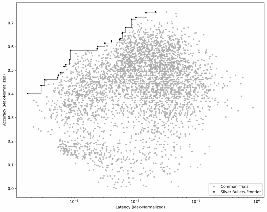
Determine 1 is an illustrative scatter plot – not from our experiments – exhibiting accomplished syftr optimization trials. Sub-plot A and Sub-plot B are equivalent, however B highlights the primary three Pareto-frontiers: P1 (crimson), P2 (inexperienced), and P3 (blue).
Every trial: A particular circulation configuration is evaluated on accuracy and common latency (greater accuracy, decrease latency are higher).
Pareto-frontier (P1): No different circulation has each greater accuracy and decrease latency. These are non-dominated.
Non-Pareto flows: A minimum of one Pareto circulation beats them on each metrics. These are dominated.
P2, P3: Should you take away P1, P2 turns into the next-best frontier, then P3, and so forth.
You may select between Pareto flows relying in your priorities (e.g., favoring low latency over most accuracy), however there’s no motive to decide on a dominated circulation — there’s at all times a greater possibility on the frontier.
Optimizing agentic AI flows with syftr
All through our experiments, we used syftr to optimize agentic flows for accuracy and latency.
This strategy means that you can:
Choose datasets containing query–reply (QA) pairs
Outline a search house for circulation parameters
Set targets corresponding to accuracy and value, or on this case, accuracy and latency
In brief, syftr automates the exploration of circulation configurations towards your chosen targets.
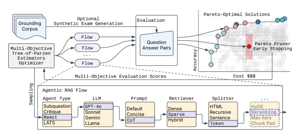
Determine 2 exhibits the high-level syftr structure.
Determine 2: Excessive-level syftr structure. For a set of QA pairs, syftr can mechanically discover agentic flows utilizing multi-objective Bayesian optimization by evaluating circulation responses with precise solutions.
Given the virtually limitless variety of attainable agentic circulation parametrizations, syftr depends on two key strategies:
Multi-objective Bayesian optimization to navigate the search house effectively.
ParetoPruner to cease analysis of probably suboptimal flows early, saving time and compute whereas nonetheless surfacing the simplest configurations.
Silver bullet experiments
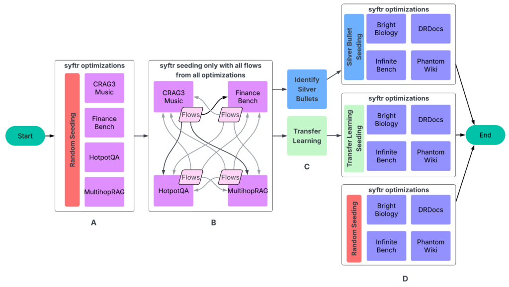
Our experiments adopted a four-part course of (Determine 3).
Determine 3: The workflow begins with a two-step information era part: A: Run syftr utilizing easy random sampling for seeding. B: Run all completed flows on all different experiments. The ensuing information then feeds into the subsequent step. C: Figuring out silver bullets and conducting switch studying. D: Operating syftr on 4 held-out datasets 3 times, utilizing three totally different seeding methods.
Step 1: Optimize flows per dataset
We ran a number of hundred trials on every of the next datasets:
CRAG Process 3 Music
FinanceBench
HotpotQA
MultihopRAG
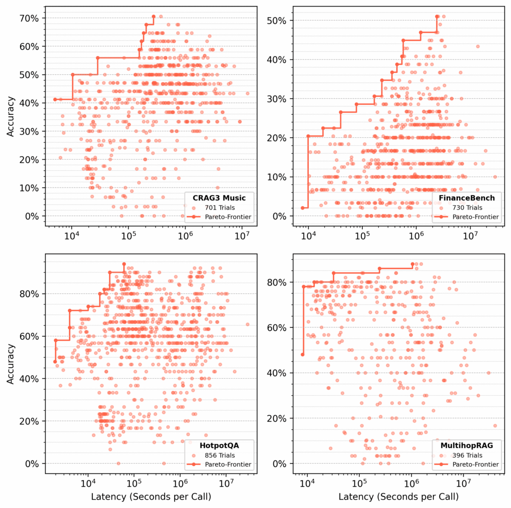
For every dataset, syftr looked for Pareto-optimal flows, optimizing for accuracy and latency (Determine 4).
Determine 4: Optimization outcomes for 4 datasets. Every dot represents a parameter mixture evaluated on 50 QA pairs. Purple traces mark Pareto-frontiers with the perfect accuracy–latency tradeoffs discovered by the TPE estimator.
Step 3: Establish silver bullets
As soon as we had equivalent flows throughout all coaching datasets, we might pinpoint the silver bullets — the flows which are Pareto-optimal on common throughout all datasets.
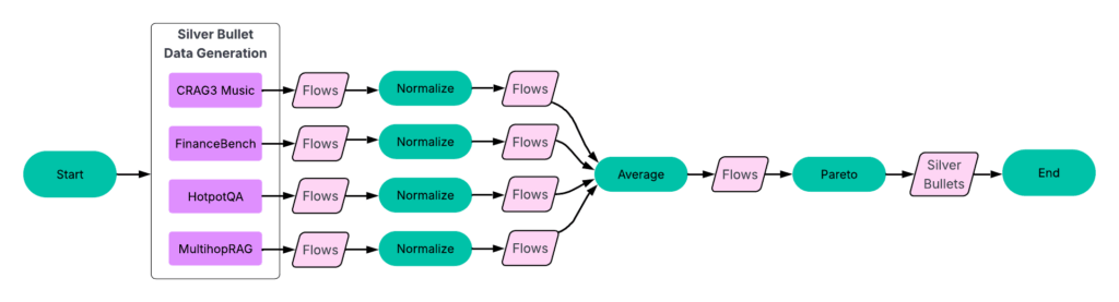
Determine 5: Silver bullet era course of, detailing the “Establish Silver Bullets” step from Determine 3.
Course of:
Normalize outcomes per dataset. For every dataset, we normalize accuracy and latency scores by the very best values in that dataset.
Group equivalent flows. We then group matching flows throughout datasets and calculate their common accuracy and latency.
Establish the Pareto-frontier. Utilizing this averaged dataset (see Determine 6), we choose the flows that construct the Pareto-frontier.
These 23 flows are our silver bullets — those that carry out properly throughout all coaching datasets.
Determine 6: Normalized and averaged scores throughout datasets. The 23 flows on the Pareto-frontier carry out properly throughout all coaching datasets.
Step 4: Seed with switch studying
In our authentic syftr paper, we explored switch studying as a approach to seed optimizations. Right here, we in contrast it straight towards silver bullet seeding.
On this context, switch studying merely means deciding on particular high-performing flows from historic (coaching) research and evaluating them on held-out datasets. The information we use right here is similar as for silver bullets (Determine 3).
Course of:
Choose candidates. From every coaching dataset, we took the top-performing flows from the highest two Pareto-frontiers (P1 and P2).
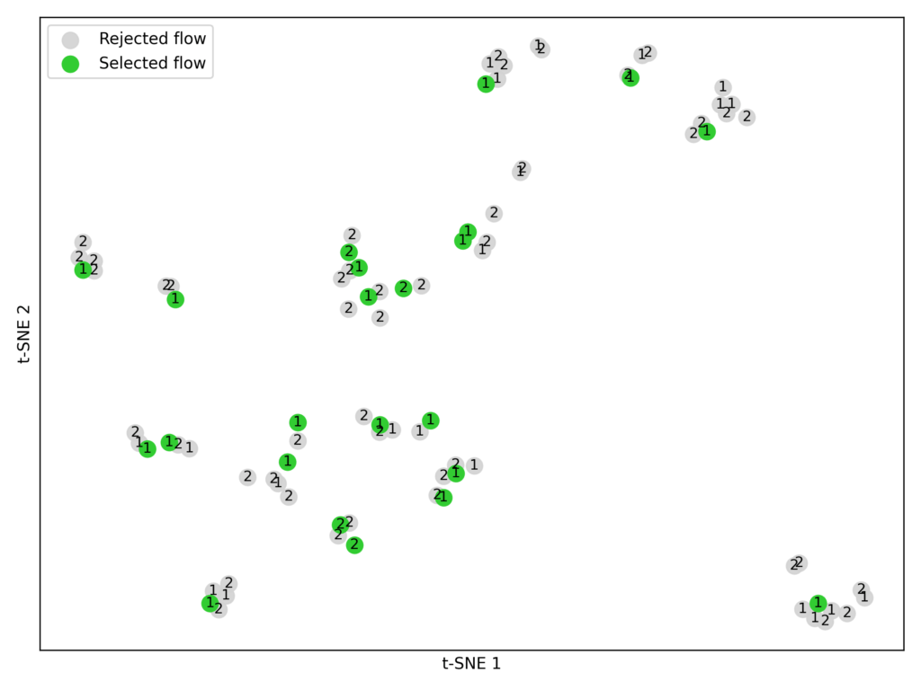
Embed and cluster. Utilizing the embedding mannequin BAAI/bge-large-en-v1.5, we transformed every circulation’s parameters into numerical vectors. We then utilized Ok-means clustering (Ok = 23) to group comparable flows (Determine 7).
Match experiment constraints. We restricted every seeding technique (silver bullets, switch studying, random sampling) to 23 flows for a good comparability, since that’s what number of silver bullets we recognized.
Observe: Switch studying for seeding isn’t but totally optimized. We might use extra Pareto-frontiers, choose extra flows, or strive totally different embedding fashions.
Determine 7: Clustered trials from Pareto-frontiers P1 and P2 throughout the coaching datasets.
Step 5: Testing all of it
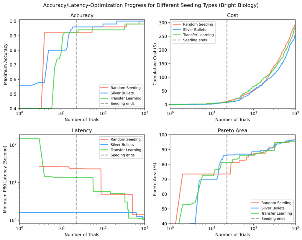
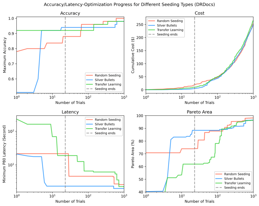
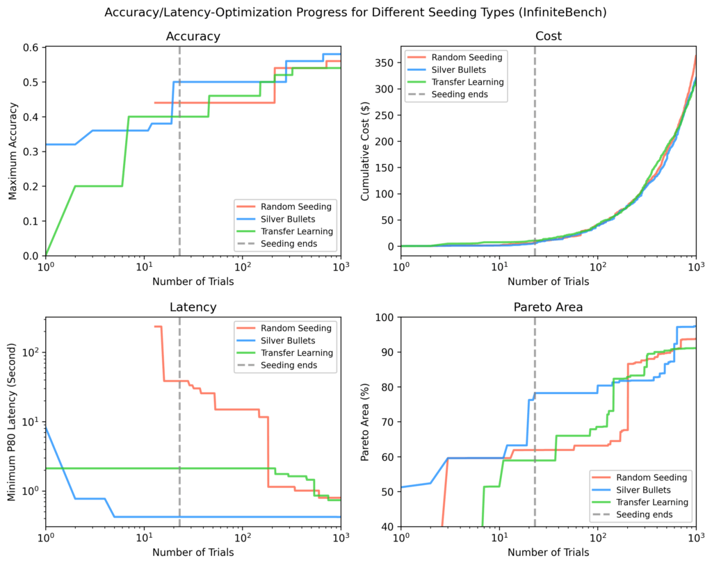
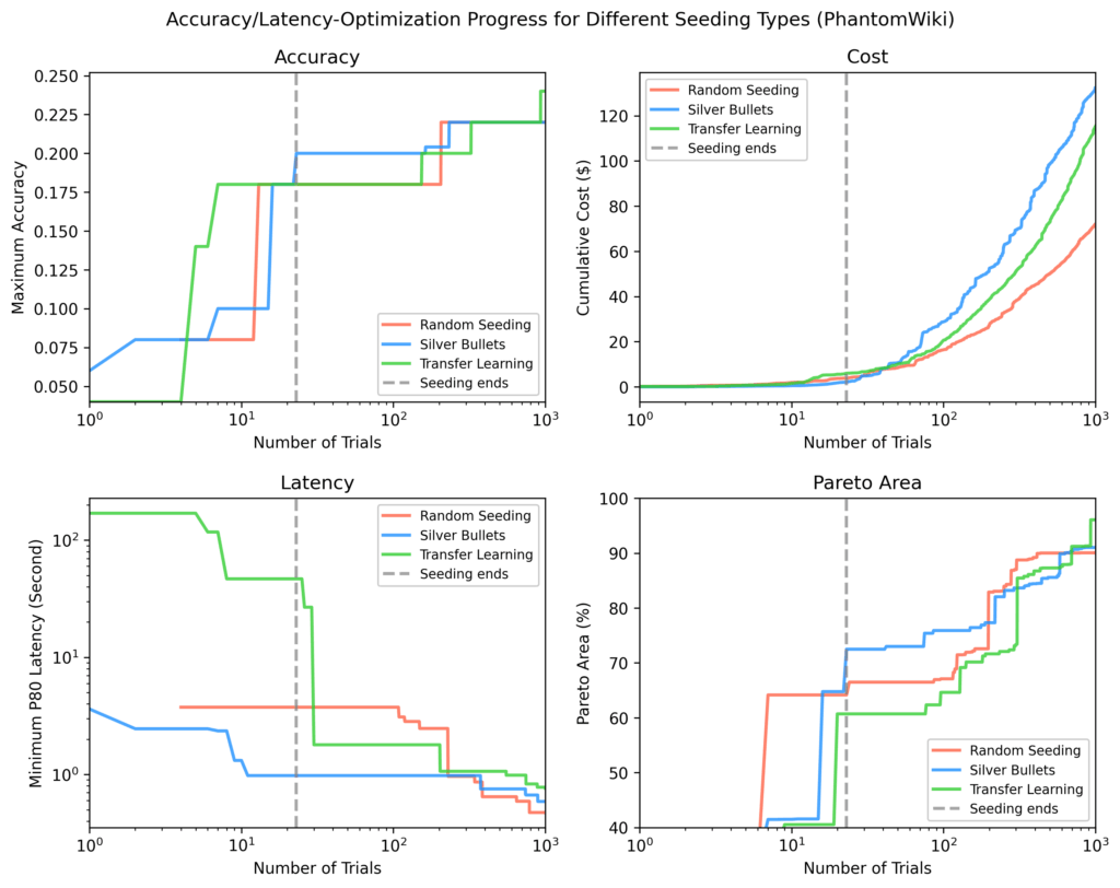
Within the ultimate analysis part (Step D in Determine 3), we ran ~1,000 optimization trials on 4 take a look at datasets — Vibrant Biology, DRDocs, InfiniteBench, and PhantomWiki — repeating the method 3 times for every of the next seeding methods:
Silver bullet seeding
Switch studying seeding
Random sampling
For every trial, GPT-4o-mini served because the decide, verifying an agent’s response towards the ground-truth reply.
Outcomes
We got down to reply:
Which seeding strategy — random sampling, switch studying, or silver bullets — delivers the perfect efficiency for a brand new dataset within the fewest trials?
For every of the 4 held-out take a look at datasets (Vibrant Biology, DRDocs, InfiniteBench, and PhantomWiki), we plotted:
Accuracy
Latency
Value
Pareto-area: a measure of how shut outcomes are to the optimum outcome
In every plot, the vertical dotted line marks the purpose when all seeding trials have accomplished. After seeding, silver bullets confirmed on common:
9% greater most accuracy
84% decrease minimal latency
28% bigger Pareto-area
in comparison with the opposite methods.
Vibrant Biology
Silver bullets had the very best accuracy, lowest latency, and largest Pareto-area after seeding. Some random seeding trials didn’t end. Pareto-areas for all strategies elevated over time however narrowed as optimization progressed.
Determine 8: Vibrant Biology outcomes
DRDocs
Just like Vibrant Biology, silver bullets reached an 88% Pareto-area after seeding vs. 71% (switch studying) and 62% (random).
Determine 9: DRDocs outcomes
InfiniteBench
Different strategies wanted ~100 extra trials to match the silver bullet Pareto-area, and nonetheless didn’t match the quickest flows discovered by way of silver bullets by the top of ~1,000 trials.
Determine 10: InfiniteBench outcomes
PhantomWiki
Silver bullets once more carried out finest after seeding. This dataset confirmed the widest price divergence. After ~70 trials, the silver bullet run briefly targeted on dearer flows.
Determine 11: PhantomWiki outcomes
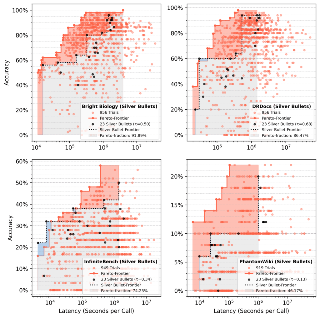
Pareto-fraction evaluation
In runs seeded with silver bullets, the 23 silver bullet flows accounted for ~75% of the ultimate Pareto-area after 1,000 trials, on common.
Purple space: Good points from optimization over preliminary silver bullet efficiency.
Blue space: Silver bullet flows nonetheless dominating on the finish.
Determine 12: Pareto-fraction for silver bullet seeding throughout all datasets
Our takeaway
Seeding with silver bullets delivers constantly sturdy outcomes and even outperforms switch studying, regardless of that methodology pulling from a various set of historic Pareto-frontier flows.
For our two targets (accuracy and latency), silver bullets at all times begin with greater accuracy and decrease latency than flows from different methods.
In the long term, the TPE sampler reduces the preliminary benefit. Inside a number of hundred trials, outcomes from all methods usually converge, which is anticipated since every ought to ultimately discover optimum flows.
So, do agentic flows exist that work properly throughout many use instances? Sure — to a degree:
On common, a small set of silver bullets recovers about 75% of the Pareto-area from a full optimization.
Efficiency varies by dataset, corresponding to 92% restoration for Vibrant Biology in comparison with 46% for PhantomWiki.
Backside line: silver bullets are an affordable and environment friendly approach to approximate a full syftr run, however they aren’t a substitute. Their influence might develop with extra coaching datasets or longer coaching optimizations.
Right here’s the total record of all 23 silver bullets, sorted from low accuracy / low latency to excessive accuracy / excessive latency: silver_bullets.json.
Attempt it your self
Wish to experiment with these parametrizations? Use the running_flows.ipynb pocket book in our syftr repository — simply ensure you have entry to the fashions listed above.
For a deeper dive into syftr’s structure and parameters, try our technical paper or discover the codebase.
Working out of area in your system, or simply want a easy solution to maintain every little thing backed up? The Western Digital Parts Transportable 2TB Exterior Onerous Drive is right here to present you peace of thoughts. And proper now, you possibly can decide one up for simply $64.99 (MSRP $79.99).
This light-weight, transportable drive makes it simple to hold your most necessary information—whether or not it’s work tasks, college paperwork, or an ever-growing photograph and video library.
And since reliability issues, WD backs it up with a three-year restricted producer guarantee.
SuperSpeed USB 3.2 Gen 1 (5Gbps): Quick, seamless transfers
Plug-and-Play expandability: Add area immediately—no setup required
Eco-friendly: Over 50% recycled supplies, recyclable packaging
Transportable design: Compact and light-weight for journey or each day use
Constructed for reliability: Backed by WD’s trusted know-how + three-year guarantee
Should you’ve been which means to unlock area, maintain a dependable backup, or simply need peace of thoughts, this supply is likely one of the best tech wins of the season.
An ADHD prognosis means an individual is liable to impulsivity and distractibility, which may manifest within the type of substance misuse, site visitors accidents, criminality and even suicidal habits.
A latest research printed within the British Medical Journal has proven that medicines like methylphenidate (model title Ritalin) can considerably scale back these dangerous outcomes in newly recognized sufferers.
The primary years after an ADHD prognosis could be a bumpy trip, bringing a way of validation and reduction, together with new challenges in determining find out how to handle newfound neurodivergence.
Globally, about 5 % of kids and a pair of.5 % of adults have ADHD. For a lot of, the way in which their brains work means they battle with duties that require focus and planning, which, on the decrease finish, means day by day stress and inconvenience.
The brand new research provides additional proof that these medicine can sort out among the most severe outcomes folks with ADHD face.
Researchers from the Karolinska Institute in Stockholm, Sweden led the research, drawing on information from 148,581 sufferers, starting from 6 to 64-years-old, who obtained an ADHD prognosis between 2007 and 2018.
Sufferers who began drug therapy (about 57 %) inside three months of prognosis noticed decreased danger throughout a lot of the severe outcomes assessed. In about 88 % of instances, the drug they took was methylphenidate.
Medicine decreased the danger of first-time substance misuse by 15 %, and recurrent misuse by 25 %.
It decreased first-time suicidal habits by 17 %, and subsequent suicide makes an attempt by 15 %.
First cases of prison habits had been decreased by 13 %, and repeat cases, by 25 %.
In addition they discovered medicine decreased the danger of first-time site visitors accidents by 12 %, and recurrent occasions by 16 %.
“Oftentimes there isn’t any info on what the dangers are for those who do not deal with ADHD,” research creator and psychiatrist Samuele Cortese, from the College of Southampton, advised journalist Philippa Roxby on the BBC.
“Now we have now proof they [ADHD medications] can scale back these dangers.”
Who would have thought that a whole e-book dedicated to the bias-variance tradeoff would make it to the NY Occasions enterprise greatest vendor record? The e-book is the recently-published Noise, by Daniel Kahneman, Olivier Sibony and Cass R. Sunstein, and, as of the start of August, it was #2 on the record. Kahneman, who wrote the influential e-book, Considering, Quick and Gradual(2011), is a grasp at relating generally summary statistical ideas to put audiences and actual world eventualities. With the bias-variance tradeoff he has set himself and his co-authors a worthy problem.
Bias in human estimation and judgment was the important thing subject in Considering, Quick and Gradual. Now, a decade later, it’s only pure that Kahneman would flip his consideration to variance, or, as he phrases it, noise.
Noise was impressed by in depth proof gathered on the variability in prison sentencing. In research of each actual and hypothetical prison circumstances, particular person judges differed by orders of magnitude within the lengths of sentences assigned to defendants. The ensuing inconsistency appears manifestly unfair.
The authors additionally recount how totally different underwriters present broadly differing insurance coverage danger assessments. These assessments are encapsulated in worth quotes which are the core of the insurance coverage enterprise: too low, and also you make no revenue, or perhaps even incur a loss. Too excessive, and also you may lose the enterprise.
Kahneman, Sibony and Sunstein make a number of factors regarding these judgment “errors:”
●Bias, the error of being constantly off-target, is extra simply visualized and receives extra standard consideration than variance. ●Error ensuing from variance might be simply as expensive as that from bias, usually extra so. ●Error from variance can usually be quantified in conditions the place error from bias can’t, for the reason that “true” worth, wanted to calculate bias, just isn’t absolutely identified (equivalent to the chance of loss for a brand new insurance coverage consumer or the suitable sentence for a criminal offense).
They go on to point out how “noise audits” can quantify the loss from noise and scale back or mitigate it. Right here, their viewers is especially enterprise, the place persons are supremely involved with quantifying worth in a uniformly accepted unit (cash), fairly in a position to act as a unified group, and fewer tousled in politics than these energetic in, say, prison justice.
As with Kahneman’s earlier work, Noise does a priceless service in explaining statistical ideas to a lay viewers. Extra importantly, it reveals knowledge scientists and statisticians the place their work suits within the scheme of sensible determination making, an all too uncommon ability in these professions. All the identical, even essentially the most devoted aficionados of statistics in apply will doubtless discover their consideration flagging earlier than reaching the midpoint on this tome. Though essential, variability as an idea for the lay viewers wants solely the primary third of the e-book. General, sadly, Noise is missing one other key statistical high quality: parsimony.


: A Assessment of Python Necessities")