Synthetic intelligence has moved past experimentation — it’s powering search engines like google and yahoo, recommender programs, monetary fashions, and autonomous automobiles. But one of many greatest hurdles standing between promising prototypes and manufacturing impression is deploying fashions safely and reliably. Current analysis notes that whereas 78 p.c of organizations have adopted AI, solely about 1 p.c have achieved full maturity. That maturity requires scalable infrastructure, sub‑second response instances, monitoring, and the flexibility to roll again fashions when issues go improper. With the panorama evolving quickly, this text affords a use‑case pushed compass to choosing the fitting deployment technique on your AI fashions. It attracts on business experience, analysis papers, and trending conversations throughout the net whereas highlighting the place Clarifai’s merchandise naturally match.

Fast Digest: What are the most effective AI deployment methods at this time?

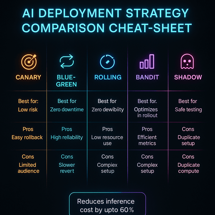
If you need the brief reply: There isn’t any single finest technique. Deployment methods equivalent to shadow testing, canary releases, blue‑inexperienced rollouts, rolling updates, multi‑armed bandits, serverless inference, federated studying, and agentic AI orchestration all have their place. The best method depends upon the use case, the threat tolerance, and the want for compliance. For instance:

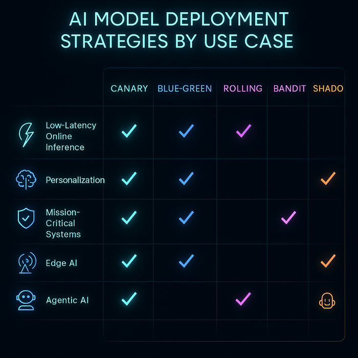
• Actual‑time, low‑latency providers (search, adverts, chat) profit from shadow deployments adopted by canary releases to validate fashions on reside visitors earlier than full cutover.
• Fast experimentation (personalization, multi‑mannequin routing) might require multi‑armed bandits that dynamically allocate visitors to the most effective mannequin.
• Mission‑important programs (funds, healthcare, finance) typically undertake blue‑inexperienced deployments for fast rollback.
• Edge and privateness‑delicate purposes leverage federated studying and on‑system inference.
• Rising architectures like serverless inference and agentic AI introduce new prospects but additionally new dangers.

We’ll unpack every situation intimately, present actionable steering, and share skilled insights below each part.

Why mannequin deployment is tough (and why it issues)

Transferring from a mannequin on a laptop computer to a manufacturing service is difficult for 3 causes:

1. Efficiency constraints – Manufacturing programs should preserve low latency and excessive throughput. For a recommender system, even a few milliseconds of extra latency can cut back click on‑via charges. And as analysis exhibits, poor response instances erode person belief shortly.
2. Reliability and rollback – A brand new mannequin model might carry out properly in staging, however fails when uncovered to unpredictable actual‑world visitors. Having an instantaneous rollback mechanism is significant to restrict injury when issues go improper.
3. Compliance and belief – In regulated industries like healthcare or finance, fashions should be auditable, truthful, and secure. They have to meet privateness necessities and observe how selections are made.

Clarifai’s perspective: As a frontrunner in AI, Clarifai sees these challenges each day. The Clarifai platform affords compute orchestration to handle fashions throughout GPU clusters, on‑prem and cloud inference choices, and native runners for edge deployments. These capabilities guarantee fashions run the place they’re wanted most, with strong observability and rollback options in-built.

Professional insights

• Peter Norvig, famous AI researcher, reminds groups that “machine studying success is not only about algorithms, however about integration: infrastructure, knowledge pipelines, and monitoring should all work collectively.” Firms that deal with deployment as an afterthought typically battle to ship worth.
• Genevieve Bell, anthropologist and technologist, emphasizes that belief in AI is earned via transparency and accountability. Deployment methods that help auditing and human oversight are important for top‑impression purposes.

How does shadow testing allow secure rollouts?

Shadow testing (typically known as silent deployment or darkish launch) is a method the place the brand new mannequin receives a copy of reside visitors however its outputs aren’t proven to customers. The system logs predictions and compares them to the present mannequin’s outputs to measure variations and potential enhancements. Shadow testing is good if you wish to consider mannequin efficiency in actual circumstances with out risking person expertise.

Why it issues

Many groups deploy fashions after solely offline metrics or artificial assessments. Shadow testing reveals actual‑world habits: surprising latency spikes, distribution shifts, or failures. It lets you gather manufacturing knowledge, detect bias, and calibrate threat thresholds earlier than serving the mannequin. You’ll be able to run shadow assessments for a hard and fast interval (e.g., 48 hours) and analyze metrics throughout totally different person segments.

Professional insights

• Use a number of metrics – Consider mannequin outputs not simply by accuracy however by enterprise KPIs, equity metrics, and latency. Hidden bugs might present up in particular segments or instances of day.
• Restrict unwanted side effects – Guarantee the brand new mannequin doesn’t set off state modifications (e.g., sending emails or writing to databases). Use learn‑solely calls or sandboxed environments.
• Clarifai tip – The Clarifai platform can mirror manufacturing requests to a brand new mannequin occasion on compute clusters or native runners. This simplifies shadow testing and log assortment with out service impression.

Inventive instance

Think about you’re deploying a brand new pc‑imaginative and prescient mannequin to detect product defects on a producing line. You arrange a shadow pipeline: each picture captured goes to each the present mannequin and the brand new one. The new mannequin’s predictions are logged, however the system nonetheless makes use of the present mannequin to regulate equipment. After per week, you discover that the brand new mannequin catches defects earlier however often misclassifies uncommon patterns. You regulate the edge and solely then plan to roll out.

run canary releases for low‑latency providers

After shadow testing, the subsequent step for actual‑time purposes is usually a canary launch. This method sends a small portion of visitors – equivalent to 1 p.c – to the brand new mannequin whereas the bulk continues to make use of the steady model. If metrics stay inside predefined bounds (latency, error charge, conversion, equity), visitors progressively ramps up.

Vital particulars

1. Stepwise ramp‑up – Begin with 1 p.c of visitors and monitor metrics. If profitable, improve to five%, then 20%, and proceed till full rollout. Every step ought to cross gating standards earlier than continuing.
2. Computerized rollback – Outline thresholds that set off rollback if issues go improper (e.g., latency rises by greater than 10 %, or conversion drops by greater than 1 %). Rollbacks ought to be automated to attenuate downtime.
3. Cell‑based mostly rollouts – For world providers, deploy per area or availability zone to restrict the blast radius. Monitor area‑particular metrics; what works in a single area might not in one other.
4. Mannequin versioning & function flags – Use function flags or configuration variables to change between mannequin variations seamlessly with out code deployment.

Professional insights

• Multi‑metric gating – Knowledge scientists and product house owners ought to agree on a number of metrics for promotion, together with enterprise outcomes (click on‑via charge, income) and technical metrics (latency, error charge). Solely taking a look at mannequin accuracy may be deceptive.
• Steady monitoring – Canary assessments aren’t only for the rollout. Proceed to watch after full deployment as a result of mannequin efficiency can drift.
• Clarifai tip – Clarifai supplies a mannequin administration API with model monitoring and metrics logging. Groups can configure canary releases via Clarifai’s compute orchestration and auto‑scale throughout GPU clusters or CPU containers.

Inventive instance

Take into account a buyer help chatbot that solutions product questions. A brand new dialogue mannequin guarantees higher responses however may hallucinate. You launch it as a canary to 2 p.c of customers with guardrails: if the mannequin can’t reply confidently, it transfers to a human. Over per week, you observe common buyer satisfaction and chat length. When satisfaction improves and hallucinations stay uncommon, you ramp up visitors progressively.

Multi‑armed bandits for fast experimentation

In contexts the place you’re evaluating a number of fashions or methods and wish to optimize throughout rollout, multi‑armed bandits can outperform static A/B assessments. Bandit algorithms dynamically allocate extra visitors to raised performers and cut back exploration as they acquire confidence.

The place bandits shine

1. Personalization & rating – When you’ve gotten many candidate rating fashions or advice algorithms, bandits cut back remorse by prioritizing winners.
2. Immediate engineering for LLMs – Making an attempt totally different prompts for a generative AI mannequin (e.g., summarization kinds) can profit from bandits that allocate extra visitors to prompts yielding increased person rankings.
3. Pricing methods – In dynamic pricing, bandits can take a look at and adapt value tiers to maximise income with out over‑discounting.

Bandits vs. A/B assessments

A/B assessments allocate mounted percentages of visitors to every variant till statistically vital outcomes emerge. Bandits, nevertheless, adapt over time. They stability exploration and exploitation: making certain that every one choices are tried however specializing in people who carry out properly. This leads to increased cumulative reward, however the statistical evaluation is extra complicated.

Professional insights

• Algorithm alternative issues – Totally different bandit algorithms (e.g., epsilon‑grasping, Thompson sampling, UCB) have totally different commerce‑offs. For instance, Thompson sampling typically converges shortly with low remorse.
• Guardrails are important – Even with bandits, preserve minimal visitors flooring for every variant to keep away from prematurely discarding a probably higher mannequin. Maintain a holdout slice for offline analysis.
• Clarifai tip – Clarifai can combine with reinforcement studying libraries. By orchestrating a number of mannequin variations and gathering reward indicators (e.g., person rankings), Clarifai helps implement bandit rollouts throughout totally different endpoints.

Inventive instance

Suppose your e‑commerce platform makes use of an AI mannequin to suggest merchandise. You’ve three candidate fashions: Mannequin A, B, and C. As a substitute of splitting visitors evenly, you utilize a Thompson sampling bandit. Initially, visitors is break up roughly equally. After a day, Mannequin B exhibits increased click on‑via charges, so it receives extra visitors whereas Fashions A and C obtain much less however are nonetheless explored. Over time, Mannequin B is clearly the winner, and the bandit routinely shifts most visitors to it.

Blue‑inexperienced deployments for mission‑important programs

When downtime is unacceptable (for instance, in fee gateways, healthcare diagnostics, and on-line banking), the blue‑inexperienced technique is usually most well-liked. On this method, you preserve two environments: Blue (present manufacturing) and Inexperienced (the brand new model). Site visitors may be switched immediately from blue to inexperienced and again.

The way it works

1. Parallel environments – The brand new mannequin is deployed within the inexperienced setting whereas the blue setting continues to serve all visitors.
2. Testing – You run integration assessments, artificial visitors, and probably a restricted shadow take a look at within the inexperienced setting. You evaluate metrics with the blue setting to make sure parity or enchancment.
3. Cutover – As soon as you’re assured, you flip visitors from blue to inexperienced. Ought to issues come up, you’ll be able to flip again immediately.
4. Cleanup – After the inexperienced setting proves steady, you’ll be able to decommission the blue setting or repurpose it for the subsequent model.

Professionals:

• Zero downtime through the cutover; customers see no interruption.
• Instantaneous rollback capacity; you merely redirect visitors again to the earlier setting.
• Decreased threat when mixed with shadow or canary testing within the inexperienced setting.

Cons:

• Larger infrastructure price, as it’s essential to run two full environments (compute, storage, pipelines) concurrently.
• Complexity in synchronizing knowledge throughout environments, particularly with stateful purposes.

Professional insights

• Plan for knowledge synchronization – For databases or stateful programs, resolve easy methods to replicate writes between blue and inexperienced environments. Choices embody twin writes or learn‑solely durations.
• Use configuration flags – Keep away from code modifications to flip environments. Use function flags or load balancer guidelines for atomic switchover.
• Clarifai tip – On Clarifai, you’ll be able to spin up an remoted deployment zone for the brand new mannequin after which swap the routing. This reduces guide coordination and ensures that the outdated setting stays intact for rollback.

Assembly compliance in regulated & excessive‑threat domains

Industries like healthcare, finance, and insurance coverage face stringent regulatory necessities. They have to guarantee fashions are truthful, explainable, and auditable. Deployment methods right here typically contain prolonged shadow or silent testing, human oversight, and cautious gating.

Key issues

1. Silent deployments – Deploy the brand new mannequin in a learn‑solely mode. Log predictions, evaluate them to the present mannequin, and run equity checks throughout demographics earlier than selling.
2. Audit logs & explainability – Keep detailed information of coaching knowledge, mannequin model, hyperparameters, and setting. Use mannequin playing cards to doc supposed makes use of and limitations.
3. Human‑in‑the‑loop – For delicate selections (e.g., mortgage approvals, medical diagnoses), preserve a human reviewer who can override or affirm the mannequin’s output. Present the reviewer with rationalization options or LIME/SHAP outputs.
4. Compliance evaluate board – Set up an inside committee to log off on mannequin deployment. They need to evaluate efficiency, bias metrics, and authorized implications.

Professional insights

• Bias detection – Use statistical assessments and equity metrics (e.g., demographic parity, equalized odds) to establish disparities throughout protected teams.
• Documentation – Put together complete documentation for auditors detailing how the mannequin was educated, validated, and deployed. This not solely satisfies rules but additionally builds belief.
• Clarifai tip – Clarifai helps position‑based mostly entry management (RBAC), audit logging, and integration with equity toolkits. You’ll be able to retailer mannequin artifacts and logs within the Clarifai platform to simplify compliance audits.

Inventive instance

Suppose a mortgage underwriting mannequin is being up to date. The group first deploys it silently and logs predictions for hundreds of purposes. They evaluate outcomes by gender and ethnicity to make sure the brand new mannequin doesn’t inadvertently drawback any group. A compliance officer opinions the outcomes and solely then approves a canary rollout. The underwriting system nonetheless requires a human credit score officer to log off on any choice, offering an additional layer of oversight.

Rolling updates & champion‑challenger in drift‑heavy domains

Domains like fraud detection, content material moderation, and finance see fast modifications in knowledge distribution. Idea drift can degrade mannequin efficiency shortly if not addressed. Rolling updates and champion‑challenger frameworks assist deal with steady enchancment.

The way it works

1. Rolling replace – Regularly change pods or replicas of the present mannequin with the brand new model. For instance, change one duplicate at a time in a Kubernetes cluster. This avoids a giant bang cutover and lets you monitor efficiency in manufacturing.
2. Champion‑challenger – Run the brand new mannequin (challenger) alongside the present mannequin (champion) for an prolonged interval. Every mannequin receives a portion of visitors, and metrics are logged. When the challenger persistently outperforms the champion throughout metrics, it turns into the brand new champion.
3. Drift monitoring – Deploy instruments that monitor function distributions and prediction distributions. Set off re‑coaching or fall again to a less complicated mannequin when drift is detected.

Professional insights

• Maintain an archive of historic fashions – You might must revert to an older mannequin if the brand new one fails or if drift is detected. Model the whole lot.
• Automate re‑coaching – In drift‑heavy domains, you may must re‑practice fashions weekly or each day. Use pipelines that fetch contemporary knowledge, re‑practice, consider, and deploy with minimal human intervention.
• Clarifai tip – Clarifai’s compute orchestration can schedule and handle steady coaching jobs. You’ll be able to monitor drift and routinely set off new runs. The mannequin registry shops variations and metrics for straightforward comparability.

Batch & offline scoring: when actual‑time isn’t required

Not all fashions want millisecond responses. Many enterprises depend on batch or offline scoring for duties like in a single day threat scoring, advice embedding updates, and periodic forecasting. For these situations, deployment methods deal with accuracy, throughput, and determinism fairly than latency.

Widespread patterns

1. Recreate technique – Cease the outdated batch job, run the brand new job, validate outcomes, and resume. As a result of batch jobs run offline, it’s simpler to roll again if points happen.
2. Blue‑inexperienced for pipelines – Use separate storage or knowledge partitions for brand spanking new outputs. After verifying the brand new job, swap downstream programs to learn from the brand new partition. If an error is found, revert to the outdated partition.
3. Checkpointing and snapshotting – Giant batch jobs ought to periodically save intermediate states. This enables restoration if the job fails midway and hurries up experimentation.

Professional insights

• Validate output variations – Examine the brand new job’s outputs with the outdated job. Even minor modifications can impression downstream programs. Use statistical assessments or thresholds to resolve whether or not variations are acceptable.
• Optimize useful resource utilization – Schedule batch jobs throughout low‑visitors durations to attenuate price and keep away from competing with actual‑time workloads.
• Clarifai tip – Clarifai affords batch processing capabilities through its platform. You’ll be able to run giant picture or textual content processing jobs and get outcomes saved in Clarifai for additional downstream use. The platform additionally helps file versioning so you’ll be able to preserve observe of various mannequin outputs.

Edge AI & federated studying: privateness and latency

As billions of units come on-line, Edge AI has grow to be a vital deployment situation. Edge AI strikes computation nearer to the info supply, decreasing latency and bandwidth consumption and enhancing privateness. Slightly than sending all knowledge to the cloud, units like sensors, smartphones, and autonomous automobiles carry out inference domestically.

Advantages of edge AI

1. Actual‑time processing – Edge units can react immediately, which is important for augmented actuality, autonomous driving, and industrial management programs.
2. Enhanced privateness – Delicate knowledge stays on system, decreasing publicity to breaches and complying with rules like GDPR.
3. Offline functionality – Edge units proceed functioning with out community connectivity. For instance, healthcare wearables can monitor important indicators in distant areas.
4. Price discount – Much less knowledge switch means decrease cloud prices. In IoT, native processing reduces bandwidth necessities.

Federated studying (FL)

When coaching fashions throughout distributed units or establishments, federated studying permits collaboration with out shifting uncooked knowledge. Every participant trains domestically by itself knowledge and shares solely mannequin updates (gradients or weights). The central server aggregates these updates to kind a world mannequin.

Advantages: Federated studying aligns with privateness‑enhancing applied sciences and reduces the chance of knowledge breaches. It retains knowledge below the management of every group or person and promotes accountability and auditability.

Challenges: FL can nonetheless leak data via mannequin updates. Attackers might try membership inference or exploit distributed coaching vulnerabilities. Groups should implement safe aggregation, differential privateness, and strong communication protocols.

Professional insights

• {Hardware} acceleration – Edge inference typically depends on specialised chips (e.g., GPU, TPU, or neural processing items). Investments in AI‑particular chips are rising to allow low‑energy, excessive‑efficiency edge inference.
• FL governance – Be sure that members agree on the coaching schedule, knowledge schema, and privateness ensures. Use cryptographic methods to guard updates.
• Clarifai tip – Clarifai’s native runner permits fashions to run on units on the edge. It may be mixed with safe federated studying frameworks in order that fashions are up to date with out exposing uncooked knowledge. Clarifai orchestrates the coaching rounds and supplies central aggregation.

Inventive instance

Think about a hospital consortium coaching a mannequin to foretell sepsis. Resulting from privateness legal guidelines, affected person knowledge can’t go away the hospital. Every hospital runs coaching domestically and shares solely encrypted gradients. The central server aggregates these updates to enhance the mannequin. Over time, all hospitals profit from a shared mannequin with out violating privateness.

Multi‑tenant SaaS and retrieval‑augmented era (RAG)

Why multi‑tenant fashions want further care

Software program‑as‑a‑service platforms typically host many buyer workloads. Every tenant may require totally different fashions, knowledge isolation, and launch schedules. To keep away from one buyer’s mannequin affecting one other’s efficiency, platforms undertake cell‑based mostly rollouts: isolating tenants into unbiased “cells” and rolling out updates cell by cell.

Retrieval‑augmented era (RAG)

RAG is a hybrid structure that mixes language fashions with exterior information retrieval to provide grounded solutions. In response to latest studies, the RAG market reached $1.85 billion in 2024 and is rising at 49 % CAGR. This surge displays demand for fashions that may cite sources and cut back hallucination dangers.

How RAG works: The pipeline includes three elements: a retriever that fetches related paperwork, a ranker that orders them, and a generator (LLM) that synthesizes the ultimate reply utilizing the retrieved paperwork. The retriever might use dense vectors (e.g., BERT embeddings), sparse strategies (e.g., BM25), or hybrid approaches. The ranker is usually a cross‑encoder that gives deeper relevance scoring. The generator makes use of the highest paperwork to provide the reply.

Advantages: RAG programs can cite sources, adjust to rules, and keep away from costly high quality‑tuning. They cut back hallucinations by grounding solutions in actual knowledge. Enterprises use RAG to construct chatbots that reply from company information bases, assistants for complicated domains, and multimodal assistants that retrieve each textual content and pictures.

Deploying RAG fashions

1. Separate elements – The retriever, ranker, and generator may be up to date independently. A typical replace may contain enhancing the vector index or the retriever mannequin. Use canary or blue‑inexperienced rollouts for every element.
2. Caching – For standard queries, cache the retrieval and era outcomes to attenuate latency and compute price.
3. Provenance monitoring – Retailer metadata about which paperwork have been retrieved and which elements have been used to generate the reply. This helps transparency and compliance.
4. Multi‑tenant isolation – For SaaS platforms, preserve separate indices per tenant or apply strict entry management to make sure queries solely retrieve approved content material.

Professional insights

• Open‑supply frameworks – Instruments like LangChain and LlamaIndex pace up RAG growth. They combine with vector databases and enormous language fashions.
• Price financial savings – RAG can cut back high quality‑tuning prices by 60–80 % by retrieving domain-specific information on demand fairly than coaching new parameters.
• Clarifai tip – Clarifai can host your vector indexes and retrieval pipelines as a part of its platform. Its API helps including metadata for provenance and connecting to generative fashions. For multi‑tenant SaaS, Clarifai supplies tenant isolation and useful resource quotas.

Agentic AI & multi‑agent programs: the subsequent frontier

Agentic AI refers to programs the place AI brokers make selections, plan duties, and act autonomously in the actual world. These brokers may write code, schedule conferences, or negotiate with different brokers. Their promise is big however so are the dangers.

Designing for worth, not hype

McKinsey analysts emphasize that success with agentic AI isn’t concerning the agent itself however about reimagining the workflow. Firms ought to map out the top‑to‑finish course of, establish the place brokers can add worth, and guarantee individuals stay central to choice‑making. The commonest pitfalls embody constructing flashy brokers that do little to enhance actual work, and failing to offer studying loops that allow brokers adapt over time.

When to make use of brokers (and when to not)

Excessive‑variance, low‑standardization duties profit from brokers: e.g., summarizing complicated authorized paperwork, coordinating multi‑step workflows, or orchestrating a number of instruments. For easy rule‑based mostly duties (knowledge entry), rule‑based mostly automation or predictive fashions suffice. Use this guideline to keep away from deploying brokers the place they add pointless complexity.

Safety & governance

Agentic AI introduces new vulnerabilities. McKinsey notes that agentic programs current assault surfaces akin to digital insiders: they’ll make selections with out human oversight, probably inflicting hurt if compromised. Dangers embody chained vulnerabilities (errors cascade throughout a number of brokers), artificial identification assaults, and knowledge leakage. Organizations should arrange threat assessments, safelists for instruments, identification administration, and steady monitoring.

Professional insights

• Layered governance – Assign roles: some brokers carry out duties, whereas others supervise. Present human-in-the-loop approvals for delicate actions.
• Check harnesses – Use simulation environments to check brokers earlier than connecting to actual programs. Mock exterior APIs and instruments.
• Clarifai tip – Clarifai’s platform helps orchestration of multi‑agent workflows. You’ll be able to construct brokers that decision a number of Clarifai fashions or exterior APIs, whereas logging all actions. Entry controls and audit logs assist meet governance necessities.

Inventive instance

Think about a multi‑agent system that helps engineers troubleshoot software program incidents. A monitoring agent detects anomalies and triggers an evaluation agent to question logs. If the difficulty is code-related, a code assistant agent suggests fixes and a deployment agent rolls them out below human approval. Every agent has outlined roles and should log actions. Governance insurance policies restrict the assets every agent can modify.

Serverless inference & on‑prem deployment: balancing comfort and management

Serverless inferencing

In conventional AI deployment, groups handle GPU clusters, container orchestration, load balancing, and auto‑scaling. This overhead may be substantial. Serverless inference affords a paradigm shift: the cloud supplier handles useful resource provisioning, scaling, and administration, so that you pay just for what you utilize. A mannequin can course of one million predictions throughout a peak occasion and scale right down to a handful of requests on a quiet day, with zero idle price.

Options: Serverless inference contains computerized scaling from zero to hundreds of concurrent executions, pay‑per‑request pricing, excessive availability, and close to‑instantaneous deployment. New providers like serverless GPUs (introduced by main cloud suppliers) permit GPU‑accelerated inference with out infrastructure administration.

Use instances: Fast experiments, unpredictable workloads, prototypes, and price‑delicate purposes. It additionally fits groups with out devoted DevOps experience.

Limitations: Chilly begin latency may be increased; lengthy‑working fashions might not match the pricing mannequin. Additionally, vendor lock‑in is a priority. You’ll have restricted management over setting customization.

On‑prem & hybrid deployments

In response to business forecasts, extra corporations are working customized AI fashions on‑premise as a result of open‑supply fashions and compliance necessities. On‑premise deployments give full management over knowledge, {hardware}, and community safety. They permit for air‑gapped programs when regulatory mandates require that knowledge by no means leaves the premises.

Hybrid methods mix each: run delicate elements on‑prem and scale out inference to the cloud when wanted. For instance, a financial institution may preserve its threat fashions on‑prem however burst to cloud GPUs for giant scale inference.

Professional insights

• Price modeling – Perceive whole price of possession. On‑prem {hardware} requires capital funding however could also be cheaper long run. Serverless eliminates capital expenditure however may be costlier at scale.
• Vendor flexibility – Construct programs that may swap between on‑prem, cloud, and serverless backends. Clarifai’s compute orchestration helps working the identical mannequin throughout a number of deployment targets (cloud GPUs, on‑prem clusters, serverless endpoints).
• Safety – On‑prem just isn’t inherently safer. Cloud suppliers make investments closely in safety. Weigh compliance wants, community topology, and menace fashions.

Inventive instance

A retail analytics firm processes thousands and thousands of in-store digital camera feeds to detect stockouts and shopper habits. They run a baseline mannequin on serverless GPUs to deal with spikes throughout peak procuring hours. For shops with strict privateness necessities, they deploy native runners that preserve footage on website. Clarifai’s platform orchestrates the fashions throughout these environments and manages replace rollouts.

Evaluating deployment methods & choosing the proper one

There are numerous methods to select from. Here’s a simplified framework:

Step 1: Outline your use case & threat stage

Ask: Is the mannequin user-facing? Does it function in a regulated area? How expensive is an error? Excessive-risk use instances (medical analysis) want conservative rollouts. Low-risk fashions (content material advice) can use extra aggressive methods.

Step 2: Select candidate methods

1. Shadow testing for unknown fashions or these with giant distribution shifts.
2. Canary releases for low-latency purposes the place incremental rollout is feasible.
3. Blue-green for mission-critical programs requiring zero downtime.
4. Rolling updates and champion-challenger for steady enchancment in drift-heavy domains.
5. Multi-armed bandits for fast experimentation and personalization.
6. Federated & edge for privateness, offline functionality, and knowledge locality.
7. Serverless for unpredictable or cost-sensitive workloads.
8. Agentic AI orchestration for complicated multi-step workflows.

Step 3: Plan and automate testing

Develop a testing plan: collect baseline metrics, outline success standards, and select monitoring instruments. Use CI/CD pipelines and mannequin registries to trace variations, metrics, and rollbacks. Automate logging, alerts, and fallbacks.

Step 4: Monitor & iterate

After deployment, monitor metrics constantly. Observe for drift, bias, or efficiency degradation. Arrange triggers to retrain or roll again. Consider enterprise impression and regulate methods as mandatory.

Professional insights

• SRE mindset – Undertake the SRE precept of embracing threat whereas controlling blast radius. Rollbacks are regular and ought to be rehearsed.
• Enterprise metrics matter – In the end, success is measured by the impression on customers and income. Align mannequin metrics with enterprise KPIs.
• Clarifai tip – Clarifai’s platform integrates mannequin registry, orchestration, deployment, and monitoring. It helps implement these finest practices throughout on-prem, cloud, and serverless environments.

AI Mannequin Deployment Methods by Use Case

Professional Perception

• Hybrid rollouts typically mix shadow + canary, making certain high quality below manufacturing visitors earlier than full launch.
• Observability pipelines (metrics, logs, drift screens) are as important because the deployment methodology.
• For agentic AI, use audit-ready reminiscence shops and tool-call simulation earlier than manufacturing enablement.
• Clarifai Compute Orchestration simplifies canary and blue-green deployments by automating GPU routing and rollback logic throughout environments.
• Clarifai Native Runners allow on-prem or edge deployment with out importing delicate knowledge.

How Clarifai Allows Strong Deployment at Scale

Fashionable AI deployment isn’t nearly placing fashions into manufacturing — it’s about doing it effectively, reliably, and throughout any setting. Clarifai’s platform helps groups operationalize the methods mentioned earlier — from canary rollouts to hybrid edge deployments — via a unified, vendor-agnostic infrastructure.

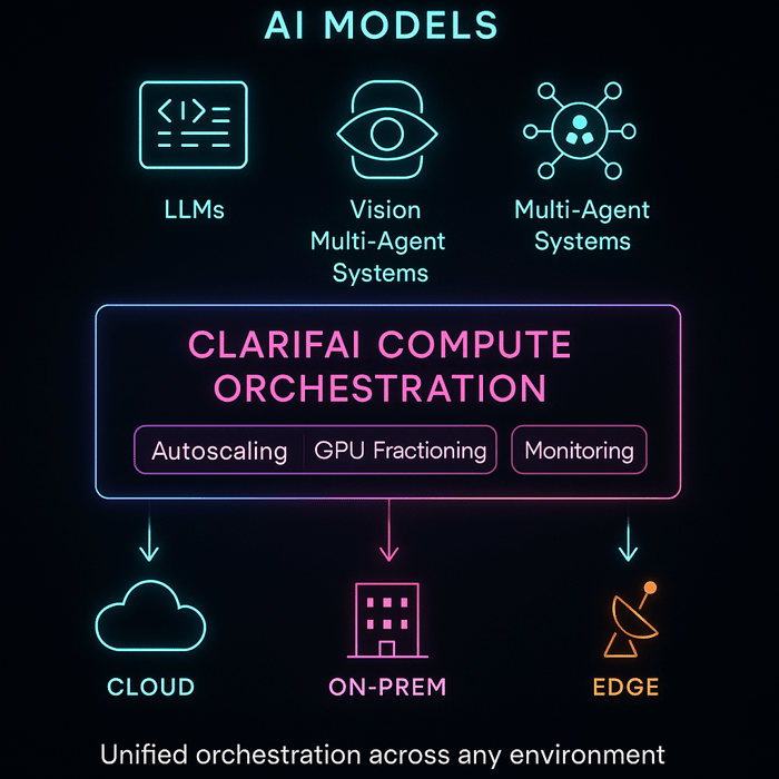
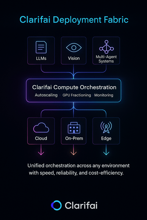
Clarifai Compute Orchestration

Clarifai’s Compute Orchestration serves as a management airplane for mannequin workloads, intelligently managing GPU assets, scaling inference endpoints, and routing visitors throughout cloud, on-prem, and edge environments.
It’s designed to assist groups deploy and iterate sooner whereas sustaining price transparency and efficiency ensures.

Key benefits:

• Efficiency & Price Effectivity: Delivers 544 tokens/sec throughput, 3.6 s time-to-first-answer, and a blended price of $0.16 per million tokens — among the many quickest GPU inference charges for its value.
• Autoscaling & Fractional GPUs: Dynamically allocates compute capability and shares GPUs throughout smaller jobs to attenuate idle time.
• Reliability: Ensures 99.999% uptime with computerized redundancy and workload rerouting — important for mission-sensitive deployments.
• Deployment Flexibility: Helps all main rollout patterns (canary, blue-green, shadow, rolling) throughout heterogeneous infrastructure.
• Unified Observability: Constructed-in dashboards for latency, throughput, and utilization assist groups fine-tune deployments in actual time.

“Our prospects can now scale their AI workloads seamlessly — on any infrastructure — whereas optimizing for price, reliability, and pace.”
— Matt Zeiler, Founder & CEO, Clarifai

AI Runners and Hybrid Deployment

For workloads that demand privateness or ultra-low latency, Clarifai AI Runners prolong orchestration to native and edge environments, letting fashions run immediately on inside servers or units whereas staying linked to the identical orchestration layer.
This permits safe, compliant deployments for enterprises dealing with delicate or geographically distributed knowledge.

Collectively, Compute Orchestration and AI Runners give groups a single deployment material — from prototype to manufacturing, cloud to edge — making Clarifai not simply an inference engine however a deployment technique enabler.

Continuously Requested Questions (FAQs)

1. What’s the distinction between canary and blue-green deployments?

Canary deployments progressively roll out the brand new model to a subset of customers, monitoring efficiency and rolling again if wanted. Blue-green deployments create two parallel environments; you narrow over all visitors without delay and might revert immediately by switching again.

2. When ought to I think about federated studying?

Use federated studying when knowledge is distributed throughout units or establishments and can’t be centralized as a result of privateness or regulation. Federated studying permits collaborative coaching whereas maintaining knowledge localized.

3. How do I monitor mannequin drift?

Monitor enter function distributions, prediction distributions, and downstream enterprise metrics over time. Arrange alerts if distributions deviate considerably. Instruments like Clarifai’s mannequin monitoring or open-source options might help.

4. What are the dangers of agentic AI?

Agentic AI introduces new vulnerabilities equivalent to artificial identification assaults, chained errors throughout brokers, and untraceable knowledge leakage. Organizations should implement layered governance, identification administration, and simulation testing earlier than connecting brokers to actual programs.

5. Why does serverless inference matter?

Serverless inference eliminates the operational burden of managing infrastructure. It scales routinely and expenses per request. Nevertheless, it might introduce latency as a result of chilly begins and might result in vendor lock-in.

6. How does Clarifai assist with deployment methods?

Clarifai supplies a full-stack AI platform. You’ll be able to practice, deploy, and monitor fashions throughout cloud GPUs, on-prem clusters, native units, and serverless endpoints. Options like compute orchestration, mannequin registry, role-based entry management, and auditable logs help secure and compliant deployments.

Conclusion

Mannequin deployment methods aren’t one-size-fits-all. By matching deployment methods to particular use instances and balancing threat, pace, and price, organizations can ship AI reliably and responsibly. From shadow testing to agentic orchestration, every technique requires cautious planning, monitoring, and governance. Rising traits like serverless inference, federated studying, RAG, and agentic AI open new prospects but additionally demand new safeguards. With the fitting frameworks and instruments—and with platforms like Clarifai providing compute orchestration and scalable inference throughout hybrid environments—enterprises can flip AI prototypes into manufacturing programs that really make a distinction.