Additionally, the inverse of the bilinear operate (a.okay.a. Möbius transformation)
is the operate
once more assuming advert − bc ≠ 0.
The elementary takeaway is that listed here are two helpful equations which can be related in look, so memorizing one makes it straightforward to memorize the opposite. We might cease there, however let’s dig slightly deeper.
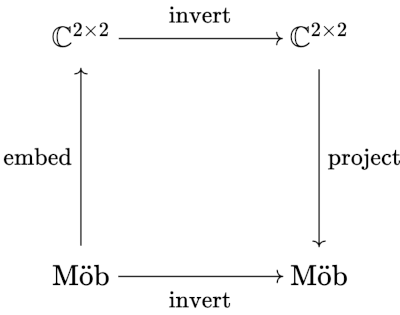
There’s apparently an affiliation between 2 × 2 matrices and Möbius transformations
This affiliation is so robust that we will use it to compute the inverse of a Möbius transformation by going to the related matrix, inverting it, and going again to a Möbius transformation. In diagram type, we now have the next
Now there are just a few lose ends. Initially, we don’t actually have a map between Möbius transformations and matrices per se; we now have a map between a explicit illustration of a Möbius transformation and a 2 × 2 matrix. If we multiplied a, b, c, and d in a Möbius transformation by 10, for instance, we’d nonetheless have the identical transformation, only a totally different illustration, however it will go to a unique matrix.
What we actually have a map between Möbius transformations and equivalence lessons of invertible matrices, the place two matrices are equal if one is a non-zero a number of of the opposite. If we wished to make the diagram above extra rigorous, we’d substitute ℂ2×2 with PL(2, ℂ), linear transformations on the advanced projective airplane. In refined phrases, our map between Möbius transformations and matrices is an isomorphism between automorphisms of the Riemann sphere and PL(2, ℂ).
Möbius transformations act loads like linear transformations as a result of they are linear transformations, however on the advanced projective airplane, not on the advanced numbers. Extra on that right here.
Get the Fashionable Science every day publication💡
Breakthroughs, discoveries, and DIY ideas despatched each weekday.
There’s a saying in corn nation: “Knee excessive by the Fourth of July.” The adage refers to a farmer’s aim for his or her crops in the event that they hope to make the October harvest. And whereas most Midwesterners are acquainted with the axiom, Tim Fitzgerald is aware of the folksy chorus misplaced its relevancy a long time in the past.
“That hasn’t truly been true since previous to fashionable fertilizers. These days corn is about six ft or taller by the Fourth of July,” Fitzgerald, a farmer in Lafayette, Indiana, tells Fashionable Science.
Fitzgerald, nevertheless, nonetheless adheres to the basic timeline. That’s as a result of his farm is not strictly within the agricultural enterprise. After a 22-year profession in industrial commerce present designing, Fitzgerald has since spent almost that lengthy overseeing “northwest Indiana’s largest corn maze,” Exploration Acres.
Business farmers usually end planting by mid-Might, however Fitzgerald’s crew begins sowing the primary week of June. By the point Fourth of July fireworks are shimmering overhead, Exploration Acres’ corn is inching in direction of your waist. The technique isn’t out of a reverence for custom, nevertheless.
“We plant later as a result of we need to have corn that’s as inexperienced as potential for so long as potential. We additionally use actually late-maturing corn that matures at round 113 days,” he explains.
As soon as Fitzgerald opens the maze in September, its winding partitions are effectively above the heads of the estimated 45,000 seasonal guests that trek its miles of pathways. However guaranteeing the correct top is just one element of the monthslong mazebuilding endeavor—a course of that’s equal components logistics, agricultural science, technological coordination, and artistry.
Exploration Acres started as a working farm with livestock within the Nineteen Twenties. Credit score: John Lumkes
The olden days
Fitzgerald was already well-suited for the labyrinth enterprise when he transitioned careers and transformed his household’s dilapidated farm right into a regional attraction in 2008. Throughout his time away, nevertheless, a lot of the almost century-old property had began to crumble.
“It was actually falling aside,” he remembers.
Because the agricultural trade continued its shift away from smaller farms to company megafacilities, locations like Exploration Acres transitioned into the agritourism enterprise. These repurposed farms provided colleges seasonal academic alternatives, in addition to the possibility to show fields into symbolic celebrations of America’s favourite money crop.
Forward of fall 2008, Fitzgerald reached out to Shawn Stolworthy at MazePlay, an Idaho-based firm specializing in all issues corn maze, to plan out his first labyrinth. The maze designs at Exploration Acres right now vary wherever from 18 to 23 acres relying on the season, however Fitzgerald settled on a relatively modest 15-acre association for the inaugural yr.
Simply as farming has modernized over time, so has the method that goes into making ready a corn maze. As Fitzgerald explains, the early technique relied on a subtractive strategy. The 1st step was to plant and develop your corn on the applicable time. In the meantime, Fitzgerald determined and created a creative theme himself. As soon as the pathways had been finalized, it was a matter of making the maze’s vector recordsdata in Adobe Illustrator. No, actually.
“MazePlay developed proprietary software program that allows you to lower mazes utilizing GPS. At the moment, it was all vector-based,” he says. “You had been mainly creating a middle line the place the paths could be, and you then used steer-track expertise on tractors that allowed the tractors to autonomously comply with the vectors. You set your floor velocity, and it goes.”
Throughout that period, a tractor’s turning radius and different components restricted the maze’s complexity. In a great world, Fitzgerald would have merely planted corn solely the place wanted and left the remaining barren for guests to stroll. It took almost a decade for the expertise to meet up with that concept. Enter: SpeedTubes.
Utilizing the SpeedTube technique, mazes could be grown with solely the corn wanted to type the paths and designs, leaving the bottom flat. Credit score: Deposit Images John Lumkes
‘Printing’ pathways
SpeedTubes are designed so farmers can customise the spacing between crops as a method to enhance progress whereas minimizing the danger of illness. However Fitzgerald and his collaborators noticed one other use for them.
“We wouldn’t want to make use of as a lot corn as a result of we wouldn’t must plant your complete area. We’ll simply plant corn the place we’d like it,” he says. “Mainly what they do is that they have this little vacuum servo on it that may maintain onto the little grain of corn till you need to drop it exactly.”
Exploration Acres started experimenting with the brand new technique in 2017. The outcomes had been instantly noticeable. As an alternative of ten seed baggage, the SpeedTube-assisted design required solely seven. (A single bag of seed can plant round two-and-a-quarter acres of corn.)
Gone had been the times of tractors plowing by a area to carve out walkways. Now, they merely roll from one facet of the acreage to a different, flip, and repeat the method. With the design keyed into the onboard software program, the velocity tubes did the remaining by dropping seeds solely the place mandatory.
“Everytime any of these rows intersect with a [maze] path, the velocity planter will flip off till it will get to the opposite facet after which it turns again on. There are literally these little LED lights on the again of the hoppers going red-to-blue, red-to-blue,” Fitzgerald says.
He likens the brand new strategy to the second everybody swapped out their dot-matrix printers for inkjets. Not that the primary yr wasn’t with out problems.
Trial and error
“It’s actually fairly easy expertise, however what we bumped into in 2017 was at any time when the tractor made a flip, it reversed route,” he remembers.
This meant that upon its return runs, all the things was off by a number of ft.
“We had a blurry picture,” says Fitzgerald.
In fact, with the seeds planted underground, the employees didn’t instantly understand the problem. It was solely after a couple of weeks when the primary child corn sprouts emerged that they observed one thing amiss.
“It created an enormous headache,” he remembers.
They finally fastened the skewed design by truly planting extra seeds at an offset distance. They then returned with the trusty tiller and eliminated the additional stalks they didn’t want.
“You’re Fashionable Science. A part of science is trial and error. You will have a speculation and also you attempt to show and disprove. So that you study issues,” he says with amusing.
With a helpful lesson discovered, Fitzgerald put the brand new system to the take a look at the next yr and made nationwide information. Keep in mind that Netflix-approved Stranger Issues corn maze in 2018? That was Exploration Acres.
“I truly needed to signal an NDA, and so they shared with me what the season was going to be about, so we initially designed a complete maze for the following season,” he says.
Different mazes have celebrated the Apollo moon touchdown, dinosaurs, zombies, pirates, and different topics. This yr marks Lafayette’s bicentennial, so Exploration Acres partnered with metropolis officers to design an ode to the city. Guests this season will wander by portraits of the city’s founder, William Digby, in addition to its Revolutionary Warfare namesake, the Marquis de Lafayette. Though 2025’s theme required a bit extra outdoors tips, there are some normal guidelines Fitzgerald retains in thoughts when sitting all the way down to plan out his subsequent creation.
“I at all times attempt to have a superb composition—a superb use of optimistic and unfavourable areas,” he says.
It’s additionally vital to rotate the maze between fields. Fitzgerald’s farm consists of 4 maze areas, at all times close to their annual pumpkin patch. When not used for the orange gourds, the employees additionally plant soybeans for the free nitrogen they produce and thus minimizing the necessity for fertilizer.
This yr’s maze theme celebrates the bicentennial of Lafayette, Indiana. Credit score: John Lumkes John Lumkes
Mapping a route ahead
After almost 20 years in operation, Exploration Acres has the maze course of all the way down to a science. However its proprietor is aware of there’ll at all times be a must experiment with new approaches. It’s inevitable because the local weather disaster continues to make its presence felt. Usually, timber on the farm have already littered the grounds with walnuts, hickory nuts, and acorns, however this yr’s prolonged drought has dried the bottom and made it a haven for pests.
“I’ve obtained rodent strain,” Fitzgerald says. “I’ve obtained voles and moles and chipmunks and squirrels. All of them digging up and consuming my tulip bulbs. There’s nothing else for them to eat, it’s been so dry.”
Then there’s the warmth. The primary few weeks of the 2025 season have seen a dramatic drop in attendees resulting from record-setting temperatures.
“That’s been a significant change since we began in 2008,” he explains. “Again then, individuals would come out and so they’d drink scorching cocoa. They’d put on mittens and gloves and a winter jacket—it’d be 38 or 40 levels out and blustery.”
Fitzgerald has even jettisoned the hay bales that usually line their wagon rides. Whereas straw is simple to sit down on for those who’re carrying lengthy pants, it’s a a lot itchier expertise in shorts.
“The worth of straw’s gone up, hardly anybody crops wheat round right here anymore. So I simply stated, ‘To heck with it,’ and put in benches within the wagons. A whole lot of issues have needed to change with time,” he says.
There may be, nevertheless, at the least one element you may depend on at Exploration Acres’ gigantic corn mazes. Regardless of how difficult the paths could appear, there’s no must get spooked if you end up rotated among the many pathways.
“We hardly ever get anybody misplaced in there. We now have an emergency path that strains the perimeter with a number of exits,” Fitzgerald assures.
Store Amazon’s Prime Day sale
We’ve hand-picked dozens of PopSci-approved offers on instruments, electronics, and extra. Seize them earlier than they’re gone.
Tengo que practicar mi español más de lo que lo practico usualmente. Se me está olvidando cómo escribir y tener una conversación en español. Entiendo los programas de televisión, movies y periódicos, pero se me dificulta escribir en español.
El problema es que no uso el español diariamente. Uso mucho el inglés. Lo uso para el trabajo, para comunicarme con amigos y colegas, y para comunicarme en la casa. Mi esposa e hija solo hablan inglés, así que no tengo mucha práctica.
Pero eso va a cambiar. He decidido escribir más y más en español, sobre todo en este weblog. Así que comencemos…
No recuerdo exactamente cuándo aprendí inglés. Como vivía en Juárez, siempre estuve expuesto al inglés de El Paso, especialmente cuando visitaba a mis primos. Ellos hablaban más inglés, y yo casi todo en español. Pero aprendí suficiente viendo programas de televisión. Fue suficiente para no batallar mucho cuando comencé a tomar clases en El Paso. Eso fue en el tercer grado de primaria.
Después de un par de meses en clases donde todos hablaban inglés, aprendí al punto de que mis calificaciones mejoraron. (Aunque no fue necesario saber inglés para matemáticas.) De ahí en adelante, fui bilingüe. Y de ahí en adelante comenzó la batalla entre el inglés y el español en mi cabeza.
Algo muy interesante sucede en mi cabeza cuando sueño. La gran mayoría de la gente en mis sueños habla español o es bilingüe. Gente que nunca me ha hablado en español lo habla perfectamente en mis sueños. Supongo que mi mente traduce todo para no batallar. Pero he notado que más y más de mis sueños incluyen conversaciones en inglés, lo cual me lleva a pensar que mi mente está cambiando.
No quiero perder la habilidad de hablar y escribir en español. Es mi lengua madre y no tiene nada que pedirle a otros lenguajes. Es un lenguaje muy bonito. Cada vez que escucho a alguien hablando en español siento algo por dentro, como si estuviera de vuelta en casa, de vuelta en Aldama o Juárez.
Y no importa qué tipo de español hablen. Puede ser el español rápido y variado del Caribe. Puede ser el español lento y claro de Colombia. O el español propio y antiguo de España. O el español chilango de la Ciudad de México. O el español del norte, de Chihuahua y Coahuila, donde decimos “i ‘eñor” en lugar de “sí señor”.
O el español mocho de la gente hispanohablante en los Estados Unidos. La gente como yo.
At a latest seminar dinner the dialog drifted to causal inference, and I discussed my dream of at some point producing a Girl Gaga parody music video referred to as “Unhealthy Management”.
A full of life dialogue of dangerous controls ensued, throughout which I provided considered one of my favourite examples: a very good instrument is a nasty management.
To summarize that earlier put up: together with a legitimate instrumental variable as a management variable can solely amplify the bias on the coefficient for our endogenous regressor of curiosity.
When used as a management, the instrument “soaks up” the great (exogenous) variation within the endogenous regressor, abandoning solely the dangerous (endogenous) variation.
That is the other of what occurs in an instrumental variables regression, the place we use the instrument to extract solely the great variation within the endogenous regressor.
Extra typically, a “dangerous management” is a covariate that we shouldn’t regulate for when utilizing a selection-on-observables method to causal inference.
Upon listening to my IV instance, my colleague instantly requested “however what in regards to the coefficient on the instrument itself?”
This can be a nice query and one I hadn’t thought of earlier than.
Immediately I’ll offer you my reply.
This put up is a sequel, so chances are you’ll discover it useful to look at my earlier put up earlier than studying additional.
On the very finish of the put up I’ll depend on a number of primary concepts about directed acyclic graphs (DAGs).
If this materials is unfamiliar, chances are you’ll discover my remedy results slides useful.
With these caveats, I’ll do my greatest to maintain this put up comparatively self-contained.
Recap of Half I
Suppose that (X) is our endogenous regressor of curiosity within the linear causal mannequin (Y = alpha + beta X + U) the place (textual content{Cov}(X,U) neq 0) however (textual content{Cov}(Z,U) = 0), and the place (Z) is an instrumental variable that’s correlated with (X).
Now think about the inhabitants linear regression of (Y) on each (X) and (Z), particularly [
Y = gamma_0 + gamma_X X + gamma_Z Z + eta
]
the place the error time period (eta) satisfies (textual content{Cov}(X,eta) = textual content{Cov}(Z,eta) = mathbb{E}(eta) = 0)by development.
Additional outline the inhabitants linear regression of (X) on (Z), particularly [
X = pi_0 + pi_Z Z + V
]
the place the error time period (V) satisfies (textual content{Cov}(Z,V) = mathbb{E}(V) = 0)by development.
Lastly, outline the inhabitants linear regression of (Y) on (X) as [
Y = delta_0 + delta_X X + epsilon, quad text{Cov}(X,epsilon) = mathbb{E}(epsilon) = 0.
]
Utilizing this notation, the consequence from my earlier put up will be written as [
delta_X = beta + frac{text{Cov}(X,U)}{text{Var}(X)}, quad text{and} quad gamma_X = beta + frac{text{Cov}(X,U)}{text{Var}(V)}.
]
To grasp what this tells us, discover that, utilizing the “first-stage” regression of (X) on (Z), we will write [
text{Var}(V) equiv text{Var}(X – pi_0 – pi_Z Z) = text{Var}(X) – pi_Z^2 text{Var}(Z).
]
This reveals that each time (Z) is a related instrument ((pi_Z neq 0)), we will need to have (textual content{Var}(V) < textual content{Var}(X)).
It follows that (gamma_X) is extra biased than (delta_X): including (Z) as a management regressor solely makes our estimate of the impact of (X)worse!
What about (gamma_Z)?
So if (Z) soaks up the good variation in (X), what in regards to the coefficient (gamma_Z) on the instrument (Z)?
Maybe this coefficient incorporates some helpful details about the causal impact of (X) on (Y)?
To seek out out, we’ll use the FWL Theorem as follows: [
gamma_Z = frac{text{Cov}(Y,tilde{Z})}{text{Var}(tilde{Z})}
]
the place (Z = lambda_0 + lambda_X X + tilde{Z}) is the inhabitants linear regression of (Z) on (X).
That is the reverse of the first-stage regression of (X) on (Z) described above.
Right here the error time period (tilde{Z}) satisfies (mathbb{E}(tilde{Z}) = textual content{Cov}(tilde{Z}, X) = 0)by development.
Substituting the causal mannequin provides [
text{Cov}(Y, tilde{Z}) = text{Cov}(alpha + beta X + U, tilde{Z}) = beta text{Cov}(X,tilde{Z}) + text{Cov}(U,tilde{Z}) = text{Cov}(U, tilde{Z})
]
since (textual content{Cov}(X,tilde{Z}) = 0) by development.
Now, substituting the definition of (tilde{Z}), [
text{Cov}(U, tilde{Z}) = text{Cov}(U, Z – lambda_0 – lambda_X X) = text{Cov}(U,Z) – lambda_X text{Cov}(U,X) = -lambda_X text{Cov}(X,U)
]
since (textual content{Cov}(U,Z) = 0) by assumption.
We are able to already see that (gamma_Z) is not going to assist us find out about (beta).
Initially, the time period containing (beta) vanished; second of all, the time period that remained is polluted by the endogeneity of (X), particularly (textual content{Cov}(X,U)).
Nonetheless, let’s see if we will get a clear expression for (gamma_Z).
To date now we have calculated the numerator of the FWL expression, displaying that (textual content{Cov}(Y,tilde{Z}) = -lambda_X textual content{Cov}(X,U)).
The following step is to calculate (textual content{Var}(tilde{Z})): [
text{Var}(tilde{Z}) = text{Var}(Z – lambda_0 – lambda_X X) = text{Var}(Z) + lambda_X^2 text{Var}(X) – 2lambda_X text{Cov}(X,Z).
]
Since (lambda_X equiv textual content{Cov}(X,Z)/textual content{Var}(X)), our expression for (textual content{Var}(tilde{Z})) simplifies to [
text{Var}(tilde{Z}) = text{Var}(Z) – lambda_X text{Cov}(X,Z)
]
so now we have found that: [
gamma_Z = frac{-lambda_X text{Cov}(X,U)}{text{Var}(Z) – lambda_X text{Cov}(X,Z)}.
]
Name me old school, however I actually don’t like having (lambda_X) in that expression.
I’d really feel a lot happier if we may discover a solution to re-write this by way of the extra acquainted IV first-stage coefficient (pi_Z).
Let’s give it a strive!
Let’s use my favourite trick of multiplying by one: [
lambda_X equiv frac{text{Cov}(X,Z)}{text{Var}(X)} = frac{text{Cov}(X,Z)}{text{Var}(X)} cdot frac{text{Var}(Z)}{text{Var}(Z)} = pi_Z cdot frac{text{Var}(Z)}{text{Var}(X)}.
]
Substituting for (lambda_X) provides [
gamma_Z = frac{-pi_Z frac{text{Var}(Z)}{text{Var}(X)} text{Cov}(X,U)}{text{Var}(Z) – pi_Z frac{text{Var}(Z)}{text{Var}(X)} text{Cov}(X,Z)} = frac{-pi_Z text{Cov}(X,U)}{text{Var}(X) – pi_Z^2 text{Var}(Z)}.
]
We are able to simplify this even additional by substituting (textual content{Var}(V) = textual content{Var}(X) – pi_Z^2 textual content{Var}(Z)) from above to acquire [
gamma_Z = -pi_Z frac{text{Cov}(X,U)}{text{Var}(V)}.
]
And now we acknowledge one thing from above: (textual content{Cov}(X,U)/textual content{Var}(V)) was the bias of (gamma_X) relative to the true causal impact (beta)!
This implies we will additionally write (gamma_Z = -pi_Z (gamma_X – beta)).
A Little Simulation
We appear to be doing an terrible lot of algebra on this weblog these days.
To be sure that we haven’t made any foolish errors, let’s test our work utilizing a bit of simulation experiment taken from my earlier put up.
Spoiler alert: all the pieces checks out!
set.seed(1234)
n <- 1e5

# Simulate instrument (z)
z <- rnorm(n)

# Simulate error phrases (u, v)
library(mvtnorm)
Rho <- matrix(c(1, 0.5,
                0.5, 1), 2, 2, byrow = TRUE)
errors <- rmvnorm(n, sigma = Rho)

# Simulate linear causal mannequin
u <- errors[, 1]
v <- errors[, 2]
x <- 0.5 + 0.8 * z + v
y <- -0.3 + x + u

# Regression of y on x and z
gamma <- lm(y ~ x + z) |>
  coefficients()

gamma
## (Intercept)           x           z
##  -0.5471213   1.5018705  -0.3981116
# First-stage regression of x on z
pi <- lm(x ~ z) |>
  coefficients()

pi
## (Intercept)           z
##   0.5020338   0.7963889
# Examine two completely different expressions for gamma_Z to the estimate itself
c(gamma_z = unname(gamma[3]),
  version1 = unname(-0.8 * cov(x, u) / var(v)),
  version2 = unname(-pi[2] * (gamma[2] - 1))
)
To date all we’ve performed is horrible, tedious algebra and a bit of simulation to test that it’s appropriate.
However in actual fact there’s some very attention-grabbing instinct for the outcomes we’ve obtained, instinct that’s deeply related to the concept of a nasty management in a directed acyclic graph (DAG).
Within the mannequin we’ve described above, (Z) has a causal impact on (Y).
It is because (Z) causes (X) which in flip causes (Y).
As a result of (Z) is an instrument, its solely impact on (Y) goes by way of (X).
The unobserved confounder (U) is a standard reason for (X) and (Y) however is unrelated to (Z).
Even should you’re not accustomed to DAGs, you’ll most likely discover this diagram comparatively intuitive:
library(ggdag)
library(ggplot2)

iv_dag <- dagify(
  Y ~ X + U,
  X ~ Z + U,
  coords = record(
    x = c(Z = 1, X = 3, U = 4, Y = 5),
    y = c(Z = 1, X = 1, U = 2, Y = 1)
  )
)

iv_dag |>
  ggdag() +
  theme_dag()
Within the determine, an arrow from (A) to (B) signifies that (A) is a reason for (B).
A causal path, is a sequence of arrows that “obeys one-way indicators” and leads from (A) to (B).
As a result of there’s a directed path from (Z) to (Y), we are saying that (Z) is a reason for (Y).
To see this utilizing our regression equations from above, substitute the IV first-stage into the linear causal mannequin to acquire [
begin{align*}
Y &= alpha + beta X + U = alpha + beta (pi_0 + pi_Z Z + V) + U
&= (alpha + beta pi_0) + beta pi_Z Z + (beta V + U).
end{align*}
]
This provides us a linear equation with (Y) on the left-hand aspect and (Z)alone on the right-hand aspect.
That is referred to as the “reduced-form” regression.
Since (textual content{Cov}(Z,U)=0) by assumption and (textual content{Cov}(Z,V) = 0) by development, the reduced-form is a bona fide inhabitants linear regression.
That signifies that regressing (Y) on (Z) will certainly give us a slope that equals (pi_Z occasions beta).
To see why the slope is a product, recall that (pi_Z) is the causal impact of (Z) on (X), the (Zrightarrow X) arrow within the diagram, whereas (beta) is the causal impact of (X) on (Y), the (X rightarrow Y) arrow within the diagram.
As a result of the one method (Z) can affect (Y) is thru (X), it is sensible that the causal impact of (Z) on (Y) is the product of those two results.
So now we see that the reduced-form coefficient (pi_Z beta) is certainly a causal impact.
How does this relate to (gamma_Z)?
Do not forget that (gamma_Z) was the coefficient on (Z) in a regression of (Y) on (Z) and (X), in different phrases a regression that adjusted for (X).
So is adjusting for (X) the precise name? Completely not!
There aren’t any back-door paths between (Z) and (Y).
Which means that we don’t have to regulate for something to study the causal impact of (Z) on (Y).
In truth adjusting for (X) is a mistake for two completely different causes.
First, (X) is a mediator on the trail (Z rightarrow X rightarrow Y).
If there have been no confounding, i.e. if (textual content{Cov}(X,U) = 0) so there is no such thing as a (Urightarrow X) arrow, adjusting for (X) would block the one causal path from (Z) to (Y).
We are able to see this in our equations from above.
Suppose that (textual content{Cov}(X,U) = 0).
Then now we have (gamma_X = beta) however (gamma_Z = 0)!
There was a useless giveaway in our derivation: the formulation for (gamma_Z) doesn’t rely on (beta) in any respect.
Second, as a result of there is confounding, adjusting for (X) creates a spurious affiliation between (Z) and (Y) by way of the back-door path (Z rightarrow X leftarrow U rightarrow Y).
As a result of (X) is a collider on the trail (Z rightarrow X leftarrow U rightarrow Y), this path begins out closed.
Adjusting for (X)opens this back-door path, making a spurious affiliation between (Z) and (Y).
To see why that is the case, suppose that (beta = 0).
On this case there may be no causal impact of (X) on (Y) and therefore no causal impact of (Z) on (Y).
But when (textual content{Cov}(X,U) neq 0), then now we have (gamma_Z neq 0)!
So if you wish to study the causal impact of (Z) on (Y), it’s not simply that (X) is a dangerous management; it’s a doubly dangerous management!
With out adjusting for (X), all the pieces is ok: the reduced-form regression of (Y) on (Z) provides us precisely what we’re after.
Epilogue
Once I confirmed this put up to a different colleague he requested me whether or not there may be any solution to find out about (beta) by combining(gamma_Z) and (gamma_X).
The reply isn’t any: the regression of (Y) on (X) and (Z) alone doesn’t comprise sufficient info.
Since [
gamma_Z = -pi_Z frac{text{Cov}(X,U)}{text{Var}(V)} quad text{and} quad gamma_X = beta + frac{text{Cov}(X,U)}{text{Var}(V)}
]
we will rearrange to acquire the next expression for (beta): [
beta = gamma_X + frac{gamma_Z}{pi_Z}
]
which we will confirm in our little simulation instance as follows:
gamma[2] + gamma[3]/pi[2]
##        x
## 1.001975
Thus, with the intention to remedy for (beta), we have to run the first-stage regression to study (pi_Z).
Software program is not what it was. That is not essentially a nasty factor, but it surely does include its personal set of challenges. Up to now, if you happen to wished to construct a characteristic, you’d must construct it from scratch, with out AI 😱 Quick ahead from the darkish ages of only a few years in the past, and we’ve a plethora of third celebration APIs at our disposal that may assist us construct options quicker and extra effectively than earlier than.
The Prevalence of Third Social gathering APIs
As software program builders, we regularly commute between “I can construct all of this myself” and “I must outsource all the pieces” so we will deploy our app quicker. These days there actually appears to be an API for nearly all the pieces:
Auth
Funds
AI
SMS
Infrastructure
Climate
Translation
The checklist goes on… (and on…)
If it is one thing your app wants, there is a good likelihood there’s an API for it. Actually, Speedy API, a well-liked API market/hub, has over 50,000 APIs listed on their platform. 283 of these are for climate alone! There are even 4 completely different APIs for Disc Golf 😳 However I digress…
Whereas we have finished a terrific job of abstracting away the complexity of constructing apps and new options, we have additionally launched a brand new set of issues: what occurs when the API goes down?
Dealing with API Down Time
Whenever you’re constructing an app that depends on third celebration dependencies, you are basically constructing a distributed system. You might have your app, and you’ve got the exterior useful resource you are calling. If the API goes down, your app is more likely to be affected. How a lot it is affected relies on what the API does for you. So how do you deal with this? There are just a few methods you may make use of:
Retry Mechanism
One of many easiest methods to deal with an API failure is to only retry the request. In spite of everything, that is the low-hanging fruit of error dealing with. If the API name failed, it would simply be a busy server that dropped your request. If you happen to retry it, it would undergo. This can be a good technique for transient errors
OpenAI’s APIs, for instance, are extraordinarily well-liked and have a restricted variety of GPUs to service requests. So it is extremely seemingly that delaying and retrying just a few seconds later will work (relying on the error they despatched again, in fact).
This may be finished in just a few other ways:
Exponential backoff: Retry the request after a sure period of time, and enhance that point exponentially with every retry.
Mounted backoff: Retry the request after a sure period of time, and maintain that point fixed with every retry.
Random backoff: Retry the request after a random period of time, and maintain that point random with every retry.
You can too attempt various the variety of retries you try. Every of those configurations will depend upon the API you are calling and if there are different methods in place to deal with the error.
Here’s a quite simple retry mechanism in JavaScript:
const delay = ms => {
returnnewPromise(fulfill => {
setTimeout(fulfill, ms);
});
};
const callWithRetry = async (fn, {validate, retries=3, delay: delayMs=2000, logger}={}) => {
let res = null;
let err = null;
for (let i = 0; i < retries; i++) {
attempt {
res = await fn();
break;
} catch (e) {
err = e;
if (!validate || validate(e)) {
if (logger) logger.error(`Error calling fn: ${e.message} (retry ${i + 1} of ${retries})`);
if (i < retries - 1) await delay(delayMs);
}
}
}
if (err) throw err;
return res;
};
If the API you are accessing has a charge restrict and your calls have exceeded that restrict, then using a retry technique is usually a good approach to deal with that. To inform if you happen to’re being charge restricted, you may verify the response headers for a number of of the next:
X-RateLimit-Restrict: The utmost variety of requests you may make in a given time interval.
X-RateLimit-Remaining: The variety of requests you’ve left within the present time interval.
X-RateLimit-Reset: The time at which the speed restrict will reset.
However the retry technique isn’t a silver bullet, in fact. If the API is down for an prolonged time period, you will simply be hammering it with requests that may by no means undergo, getting you nowhere. So what else are you able to do?
Circuit Breaker Sample
The Circuit Breaker Sample is a design sample that may assist you gracefully deal with failures in distributed methods. It is a sample that is been round for some time, and it is nonetheless related immediately. The thought is that you’ve got a “circuit breaker” that screens the state of the API you are calling. If the API is down, the circuit breaker will “journey” and cease sending requests to the API. This may also help forestall your app from losing time and sources on a service that is not obtainable.
When the circuit breaker journeys, you are able to do just a few issues:
Return a cached response
Return a default response
Return an error
This is a easy implementation of a circuit breaker in JavaScript:
On this case, the open state will return a generic error, however you may simply modify it to return a cached response or a default response.
Swish Degradation
No matter whether or not or not you employ the earlier error dealing with methods, a very powerful factor is to make sure that your app can nonetheless perform when the API is down and talk points with the person. This is named “sleek degradation.” Because of this your app ought to nonetheless have the ability to present some degree of service to the person, even when the API is down, and even when that simply means you come back an error to the tip caller.
Whether or not your service itself is an API, internet app, cellular system, or one thing else, it’s best to at all times have a fallback plan in place for when your third celebration dependencies are down. This may very well be so simple as returning a 503 standing code, or as advanced as returning a cached response, a default response, or an in depth error.
Each the UI and transport layer ought to talk these points to the person to allow them to take motion as obligatory. What’s extra irritating as an finish person? An app that does not work and does not let you know why, or an app that does not work however tells you why and what you are able to do about it?
Monitoring and Alerting
Lastly, it is essential to observe the well being of the APIs you are calling. If you happen to’re utilizing a 3rd celebration API, you are on the mercy of that API’s uptime. If it goes down, you have to learn about it. You should use a service like Ping Bot to observe the well being of the API and provide you with a warning if it goes down.
Try our hands-on, sensible information to studying Git, with best-practices, industry-accepted requirements, and included cheat sheet. Cease Googling Git instructions and really study it!
Dealing with the entire error circumstances of a downed API will be tough to do in testing and integration, so reviewing an API’s previous incidents and monitoring present incidents may also help you perceive each how dependable the useful resource is and the place your app might fall quick in dealing with these errors.
With Ping Bot’s uptime monitoring, you may see the present standing and likewise look again on the historic uptime and particulars of your dependency’s downtime, which may also help you establish why your personal app might have failed.
You can too arrange alerts to inform you when the API goes down, so you may take motion as quickly because it occurs. Have Ping Bot ship alerts to your electronic mail, Slack, Discord, or webhook to robotically alert your workforce and servers when an API goes down.
Conclusion
Third celebration APIs are an effective way to construct options rapidly and effectively, however they arrive with their very own set of challenges. When the API goes down, your app is more likely to be affected. By using a retry mechanism, circuit breaker sample, and sleek degradation, you may make sure that your app can nonetheless perform when the API is down. Monitoring and alerting may also help you keep on high of the well being of the APIs you are calling, so you may take motion as quickly as they go down.
In case you are compute-constrained, use autoregressive fashions; if you’re data-constrained, use diffusion fashions.
Motivation
Progress in AI over the previous decade has largely been pushed by scaling compute and information. The recipe from GPT-1 to GPT-5 has appeared simple: prepare a bigger mannequin on extra information, and the result’s a extra succesful system.
But a central query stays: will this recipe proceed to carry from GPT-6 to GPT-N?
Many analysts and researchers consider the reply is not any. As an illustration, Ilya Sutskever, in his NeurIPS 2024 Take a look at-of-Time Award discuss, remarked: “Compute is rising—higher algorithms, higher {hardware}, larger clusters—however information just isn’t rising. We have now only one web, the fossil gasoline of AI.”
This concern is echoed by AI forecasters, who’ve analyzed compute and information development extra systematically and concluded that compute is outpacing information at an accelerating price.
Epoch AI‘s research that extrapolates the expansion charges of web information (inventory of knowledge), dataset utilization (dataset dimension projection), and compute (measured in Chinchilla-optimal tokens). Round 2028, compute outpaces the whole accessible coaching information on the web, marking the onset of a data-constrained regime. I up to date the determine by overlaying Determine 4 and Determine 5 of their paper.
The above Determine, illustrates this rigidity by overlaying projections from EpochAI’s evaluation. Their research extrapolates historic developments in compute, dataset utilization, and internet-scale information availability. The forecast means that by round 2028, we’ll enter a data-constrained regime: much more compute will likely be accessible than there are coaching tokens to eat.
This paper addresses the problem by asking: how can we commerce off extra compute for much less information? Our central thought is to revisit the foundations of recent generative modeling and evaluate the 2 dominant paradigms for scaling AI.
Broadly, there have been two households of algorithms that formed current progress in AI:
Autoregressive fashions, popularized in 2019 within the textual content area with the GPT-2 paper.
Diffusion fashions, popularized in 2020 within the imaginative and prescient area with the DDPM paper.
Each goal to maximise the joint probability, however they differ essentially in how they factorize this joint distribution.
The success of diffusion in imaginative and prescient and autoregression in language has sparked each pleasure and confusion—particularly as every neighborhood has begun experimenting with the opposite’s paradigm.
For instance, the language neighborhood has explored diffusion on textual content:
D3PM launched discrete diffusion by way of random masking, whereas Diffusion-LM utilized steady diffusion by projecting tokens to embeddings earlier than including Gaussian noise. Since then, quite a few works have prolonged this line of analysis.
Conversely, the imaginative and prescient neighborhood has experimented with doing autoregressive modeling on photos. Fashions resembling PARTI and DALLE exemplify this method with robust outcomes.
This cross-pollination has led to even better uncertainty in robotics, the place each diffusion-based and autoregressive approaches are broadly adopted. As an example this, OpenAI Deep Analysis has compiled a listing of robotics works throughout each paradigms, highlighting the shortage of consensus within the discipline.
This ambiguity raises a elementary query: ought to we be coaching diffusion fashions or autoregressive fashions?
Fast Background:
Autoregressive language fashions:
They mannequin information distribution in a left-to-right method
Since 2021, diffusion language fashions have sparked important curiosity, with many works specializing in bettering their design and efficiency.
Numbers taken from: Sahoo etal “Easy and Efficient Masked Diffusion Language Fashions”
Within the desk above, we spotlight consultant outcomes from a well-liked work. The takeaways are as follows:
Discrete diffusion performs higher than steady diffusion on textual content.
Autoregressive fashions nonetheless obtain the strongest outcomes total.
A number of works have additionally explored the scaling habits of diffusion-based language fashions.
Nie et al report that discrete diffusion LLMs require roughly 16× extra compute than autoregressive LLMs to match the identical unfavorable log-likelihood. Comparable outcomes have been noticed in multimodal domains—for example, UniDisc finds that discrete diffusion wants about 12× extra compute than autoregression for comparable likelihoods.
Nonetheless, these outcomes conflate information and compute as a result of they’re measured in a single-epoch coaching regime. This raises an necessary ambiguity: do diffusion fashions really require 16× extra compute, or do they the truth is require 16× extra information?
On this work, we explicitly disentangle information and compute. Our objective is to review diffusion and autoregressive fashions particularly in data-constrained settings.
Our Motivation
To know why diffusion could behave in another way, let’s revisit its coaching goal.
In diffusion coaching, tokens are randomly masked and the mannequin learns to get better them. Importantly, left-to-right masking is a particular case inside this framework.
Considered this manner, diffusion could be interpreted as a type of implicit information augmentation for autoregressive coaching. As an alternative of solely studying from left-to-right sequences, the mannequin additionally advantages from many different masking methods.
And if diffusion is basically information augmentation, then its advantages needs to be most pronounced when coaching is data-bottlenecked.
This attitude explains why prior works have reported weaker outcomes for diffusion: they primarily evaluated in single-epoch settings, the place information is plentiful. In distinction, our research focuses on situations the place information is proscribed and compute could be traded off extra successfully.
Our Experiments
On this work, we prepare tons of of fashions spanning a number of orders of magnitude in mannequin dimension, information amount, and variety of coaching epochs to suit scaling legal guidelines for diffusion fashions within the data-constrained setting. We summarize a few of our key findings under.
Discovering #1:
Diffusion fashions outperform autoregressive fashions when skilled with ample compute (i.e., extra epochs & parameters). Throughout totally different distinctive information scales, we observe:
At low compute, Autoregressive fashions win.
After a specific amount of compute, efficiency matches—we name this the essential compute level.
Past this, diffusion retains bettering, whereas Autoregressive plateaus or overfits.
Every level within the determine exhibits a mannequin skilled to convergence. The x-axis exhibits the whole coaching FLOPs of that time, and the y-axis exhibits one of the best validation loss achieved by that mannequin household underneath that coaching compute price range.
Discovering #2:
Autoregressive fashions start to overfit a lot shortly, whereas diffusion exhibits no indicators of overfitting even after 10x the variety of epochs. Within the above determine, we confirmed that rising compute finally favors diffusion. However compute could be scaled in two methods: (i) Growing mannequin dimension (ii) Growing the variety of epochs Within the following plot, we separate these axes.
The coloured star marks the 1-epoch level, the place Autoregressive outperforms diffusion. The star (★) denotes one of the best loss achieved by every mannequin.
Autoregressive hits its finest across the center, then overfits.
Diffusion retains bettering and reaches its finest loss on the far proper.
Not solely does diffusion profit from extra coaching—it additionally achieves a greater ultimate loss than Autoregressive (3.51 vs. 3.71).
Discovering #3:
Diffusion fashions are considerably extra strong to information repetition than autoregressive (AR) fashions.
We present coaching curves of fashions skilled with the identical complete compute, however totally different trade-offs between distinctive information and variety of epochs.
An “epoch” right here means reusing a smaller subset of knowledge extra occasions(e.g., 4 Ep is 4 epochs whereas utilizing 25% distinctive information, 2 Ep is 2 epochs with 50% and so forth).
AR fashions start to overfit as repetition will increase—their validation loss worsens and considerably diverges at increased epoch counts.
Diffusion fashions stay secure throughout all repetition ranges, exhibiting no indicators of overfitting or diverging—even at 100 epochs.
Discovering #4:
Diffusion fashions exhibit a a lot increased half-life of knowledge reuse (R_D*) —i.e., the variety of epochs after which returns from repeating information begins to considerably diminish.
We undertake the data-constrained scaling framework launched by Muennighoff et al. of their wonderful NeurIPS paper to suit scaling legal guidelines for diffusion fashions. Whereas Muennighoff et al. discovered R_D* ~ 15 for autoregressive fashions, we discover a considerably increased worth of R_D* ~ 500 for diffusion fashions—highlighting their potential to learn from much more information repetition.
The above Determine research the Decay price of knowledge worth underneath repetition: left exhibits diffusion, center AR, and proper the typical decay price for each.
Factors are empirical outcomes (darker colour = increased FLOPs, lighter colour = decrease FLOPs; every line = mounted compute), we discover that fitted curves (represented as traces) intently match the empirical factors, indicating our scaling legal guidelines are consultant. The decay price of worth for repeated information is decrease for diffusion, reflecting its better robustness to repeating. On this experiment 100% information fraction means coaching 1 epoch with 100% distinctive information, whereas 50% means 2 epoch epoch with solely utilizing 50% distinctive information and so forth.
Discovering #5:
Muennighoff et al. confirmed that repeating the dataset as much as 4 epochs is almost as efficient as utilizing recent information for autoregressive fashions.
In distinction, we discover that diffusion fashions could be skilled on repeated information for as much as 100 epochs, whereas having repeated information virtually as efficient as recent information.
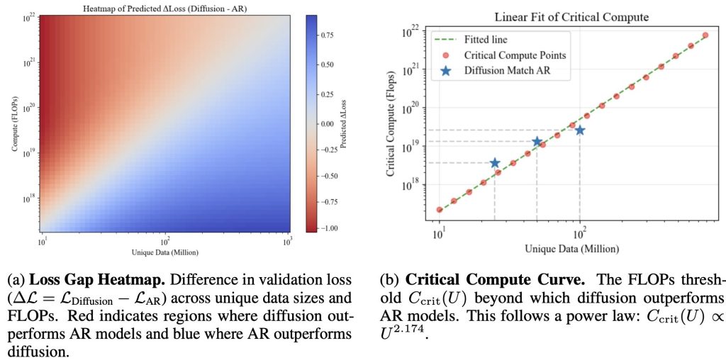
Discovering #6:
The compute required for diffusion to outperform AR follows a predictable energy legislation. Above we outlined the essential compute threshold as the quantity of FLOPs the place diffusion matches AR efficiency for a given distinctive dataset dimension.
We discover that we are able to derive a easy closed-form analytical expression for this threshold, this permits us to foretell when diffusion will surpass AR given any distinctive information dimension. Within the determine we present each the fitted curve and empirical essential threshold factors, which align intently.
Discovering #7:
The info effectivity of diffusion fashions interprets to raised downstream efficiency.
Lastly we consider the best-performing diffusion and AR fashions (skilled underneath the identical information price range) on a spread of language understanding duties.
Throughout most benchmarks, diffusion fashions outperform AR fashions, confirming that diffusion’s decrease validation loss interprets to raised downstream efficiency.
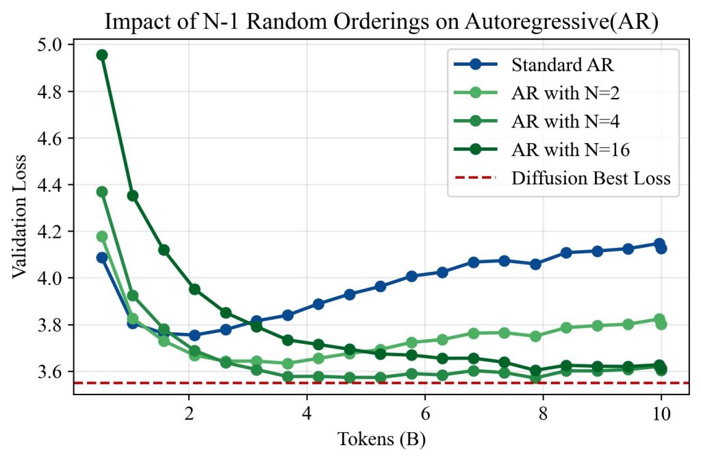
Discovering #8:
Publicity to totally different token orderings helps clarify diffusion’s information effectivity. By including express information augmentations to AR coaching, we discover that diffusion mannequin’s benefit arises from their publicity to a various set of token orderings.
As seen within the above Determine, rising N persistently lowered validation loss and delayed overfitting. At N = 16, the 100-epoch validation lack of AR fashions approached that of diffusion, suggesting that various orderings are certainly a key driver of diffusion’s information effectivity. These outcomes help our interpretation that diffusion fashions outperform AR fashions in low-data regimes as a result of they’re implicitly skilled on a richer distribution of conditional prediction duties.
Lastly, this evaluation suggests a pure continuum between the 2 paradigms: by controlling process range via masking or reordering—we might design hybrid fashions that interpolate between compute effectivity (AR-like) and information effectivity (diffusion-like).
As the provision of high-quality information plateaus, bettering information effectivity turns into important for scaling deep studying. On this work, we present that masked diffusion fashions persistently outperform autoregressive (AR) fashions in data-constrained regimes — when coaching includes repeated passes over a restricted dataset. We set up new scaling legal guidelines for diffusion fashions, revealing their potential to extract worth from repeated information far past what AR fashions can obtain.
These outcomes problem the traditional perception that AR fashions are universally superior and spotlight diffusion fashions as a compelling different when information—not compute—is the first bottleneck. Wanting forward, environment friendly use of finite information could outline the subsequent frontier in scaling deep studying fashions. Though the research have been carried out within the context of language fashions, we consider these findings ought to apply throughout any type of sequence modeling information, resembling in robotics or healthcare. For practitioners, our takeaway is straightforward: if you’re compute-constrained, use autoregressive fashions; if you’re data-constrained, use diffusion fashions.
Bibtex:
@article{prabhudesai2025diffusion,
title={Diffusion Beats Autoregressive in Information-Constrained Settings},
creator={Prabhudesai, Mihir and Wu, Mengning and Zadeh, Amir and Fragkiadaki, Katerina and Pathak, Deepak},
journal={arXiv preprint arXiv:2507.15857},
yr={2025}
}
I bear in mind the early days of my profession as a chief info safety officer (CISO). We had been typically relegated to a darkish nook of the IT division, talking a language of ports, patches, and protocols that the remainder of the C-suite politely tolerated.
It wasn’t till I discovered to translate safety gaps into enterprise danger that the dialog — and my profession — essentially modified. Now, as a CEO, I see it from the opposite facet: Safety is not only a protection mechanism; it will also be used as a strategic program for useful resource administration.
The fashionable CISO faces a basic dilemma: an overflowing toolkit, a finite price range, and a board of administrators demanding proof that “we’re protected.” Conventional approaches, reminiscent of shopping for instruments to fulfill compliance checkboxes or reacting to the most recent vendor hype, have failed. That leaves safety in a state of chaotic guesswork the place redundancy typically masks gaping holes.
The simplest answer is adopting a threat-led protection technique. This method mandates that each safety greenback, management, and gear is meticulously mapped towards the precise, real-world assault behaviors most probably to trigger the group monetary hurt. It additionally redefines the function of CISO from technical guardian to strategic danger administration accomplice. Let’s begin with why the compliance-based method of the technical guardian CISO falls quick.
Prioritizing the Proper Threats: The Adversary’s Perspective
The primary failure of the compliance-based mannequin is its lack of ability to prioritize. Not all vulnerabilities are created equal, and never all threats are related. It’s essential for an organization to evaluate and show that it’s spending cash on mitigating essentially the most vital threats, moderately than minor dangers. This apply, generally known as danger prioritization, ensures that essentially the most impactful threats are addressed first to safeguard monetary efficiency, status, and long-term viability. Losing restricted assets on insignificant dangers leaves the group weak to catastrophic — however preventable — injury.
A threat-led technique corrects this by forcing the group to undertake the next steps:
Establish the adversary. Leverage menace intelligence to establish the precise menace actors that focus on your business, geography, and technological stack.
Map techniques to property. Make the most of frameworks like MITRE ATT&CK to map the recognized techniques, strategies, and procedures (TTPs) of adversarial teams on to your group’s “crown jewels.”
Quantify the impression. Rank a TTP’s technical severity rating by potential loss expectancy.
Mapping safety instruments to danger is a strategic course of that aligns each safety management, whether or not a software or functionality, with the precise enterprise dangers it’s designed to mitigate. It shifts the safety staff’s focus from monitoring software deployment (a technical metric) to measuring the discount in monetary or operational danger (a enterprise metric).
Figuring out Protection Gaps and Instrument Redundancy
As soon as the group’s prime threats are prioritized by their monetary danger, a threat-led protection technique offers a data-driven methodology to evaluate defensive protection and expose overspending. This method permits organizations to maneuver past merely aggregating safety alerts to systematically assessing how nicely current instruments and configurations defend towards the precise threats most probably to focus on the group.
Protection gaps signify areas the place the group’s present defenses are inadequate to mitigate or detect prioritized adversarial exercise. Steady validation — the continuing verification that safety controls are working as supposed by repeatedly testing them, typically by automated simulations or assessments — is a should to remain forward of the continually altering menace and protection panorama. Assessing protection gaps permits a corporation to interchange assumptions about software effectiveness with quantifiable knowledge. This knowledge can then be used to optimize and harden defenses in weak areas.
Guiding Higher Enterprise Choice-Making
Probably the most profitable safety leaders do not simply shut gaps; they information enterprise choices by meticulously aligning each safety precedence, greenback spent, and gear bought with the group’s biggest monetary and operational dangers. A threat-led protection technique in the end offers a safety chief with the flexibility to translate technical outcomes into enterprise actions that resonate with the board and govt management — in different phrases, reframing safety from a technical situation right into a strategic enterprise enabler. Specializing in monetary impression, operational resilience, and aggressive benefit, moderately than technical jargon, helps executives perceive safety in a enterprise context. This permits them to make knowledgeable choices and align cybersecurity with broader company targets.
Not often do individuals outdoors of the safety group must know how you do safety, however they do must know the state of danger and what assets are wanted to handle it. As a substitute of reporting technical metrics, reminiscent of the typical variety of alerts their groups obtain or patching cadence, a CISO ought to current the chance hole by quantifying the chance of a business-critical failure situation. Establish, for instance, a 40% likelihood of income disruption resulting from a particular marketing campaign or vulnerability, after which argue for strategic investments that mitigate that danger.
This shift from safety funding to resilience funding empowers the board to make knowledgeable, data-driven choices about danger tolerance and strategic funding.
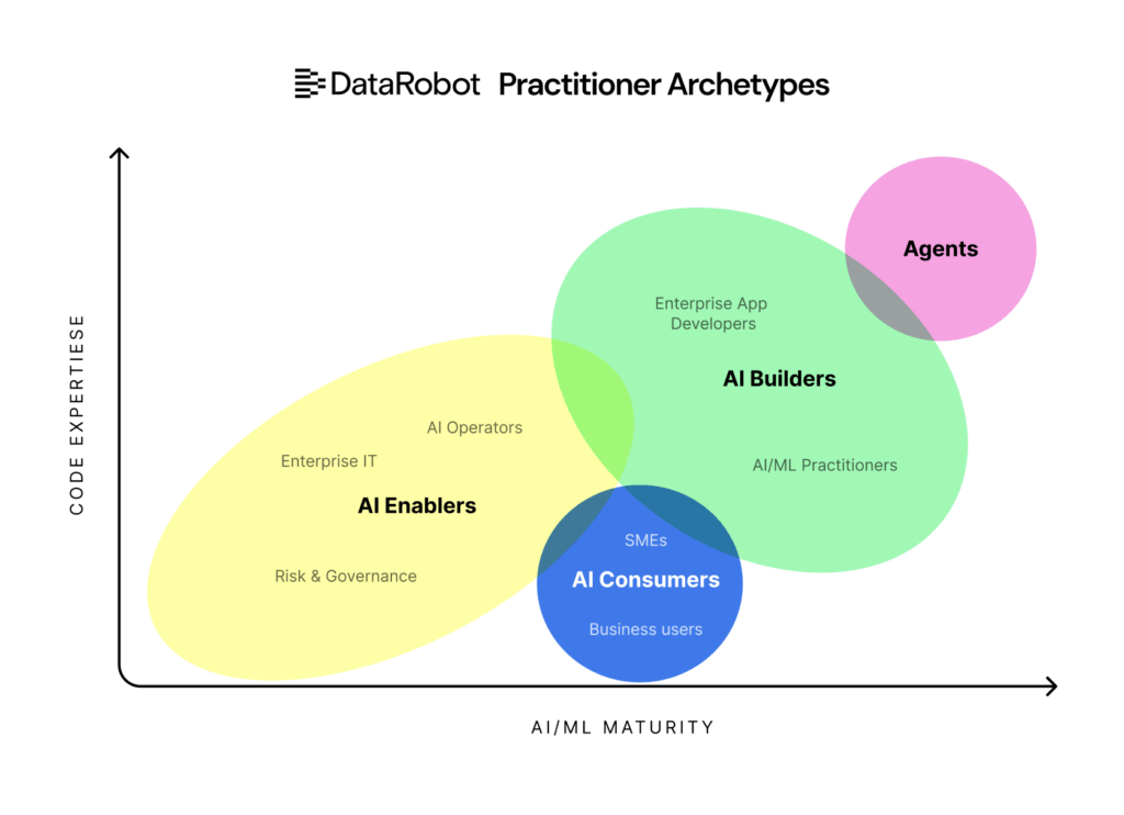
Brokers are right here. And they’re difficult most of the assumptions software program groups have relied on for many years, together with the very concept of what a “product” is.
There’s a scene in Interstellar the place the characters are on a distant, water-covered planet. Within the distance, what appears like a mountain vary seems to be huge waves steadily constructing and towering over them. With AI, it has felt a lot the identical. A large wave has been constructing on the horizon for years.
Generative AI and Vibe Coding have already shifted how design and growth occur. Now, one other seismic shift is underway: agentic AI.
The query isn’t if this wave will hit — it already has. The query is the way it will reshape the panorama enterprises thought they knew. From the vantage level of the manufacturing design crew at DataRobot, these adjustments are reshaping not simply how design is finished, but additionally long-held assumptions about what merchandise are and the way they’re constructed.
What makes agentic AI completely different from generative AI
Not like predictive or generative AI, brokers are autonomous. They make selections, take motion, and adapt to new data with out fixed human prompts. That autonomy is highly effective, however it additionally clashes with the deterministic infrastructure most enterprises depend on.
Deterministic programs anticipate the identical enter to ship the identical output each time. Brokers are probabilistic: the identical enter may set off completely different paths, selections, or outcomes. That mismatch creates new challenges round governance, monitoring, and belief.
These aren’t simply theoretical issues; they’re already enjoying out in enterprise environments.
To assist enterprises run agentic programs securely and at scale, DataRobot co-engineered the Agent Workforce Platform with NVIDIA, constructing on their AI Manufacturing unit design. In parallel, we co-developed enterprise brokers embedded instantly into SAP environments.
Collectively, these efforts allow organizations to operationalize brokers securely, at scale, and throughout the programs they already depend on.
Transferring from pilots to manufacturing
Enterprises proceed to battle with the hole between experimentation and impression. MIT analysis lately discovered that 95% of generative AI pilots fail to ship measurable outcomes — typically stalling when groups attempt to scale past proofs of idea.
Transferring from experimentation to manufacturing entails vital technical complexity. Slightly than anticipating prospects to construct every little thing from the bottom up, DataRobot shifted its strategy.
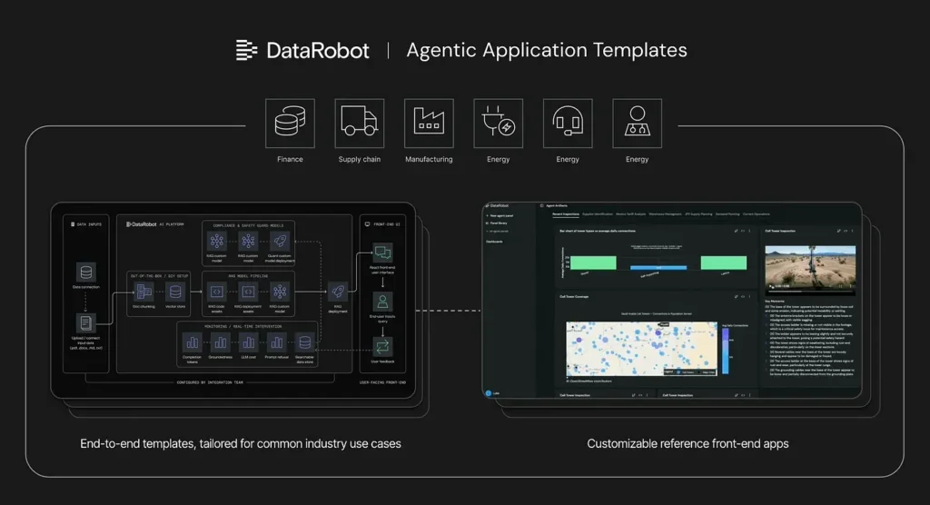
To make use of a meals analogy: as an alternative of handing prospects a pantry of uncooked components like parts and frameworks, the corporate now delivers meal kits: agent and software templates with prepped parts and confirmed recipes that work out of the field.
These templates codify finest practices throughout widespread enterprise use circumstances. Practitioners can clone them, then swap or lengthen parts utilizing the platform or their most popular instruments by way of API.
The impression: production-ready dashboards and purposes in days, not months.
Agent Workforce Platform: Use case–particular templates, AI infrastructure, and front-end integrations.
Altering how practitioners use the platform
This strategy can be reshaping how AI practitioners work together with the platform. One of many largest hurdles is creating front-end interfaces that eat the brokers and fashions: apps for forecasting demand, producing content material, retrieving information, or exploring information.
Bigger enterprises with devoted growth groups can deal with this. However smaller organizations typically depend on IT groups or AI specialists, and app growth isn’t their core ability.
To bridge that hole, DataRobot supplies customizable reference apps as beginning factors. These work nicely when the use case is an in depth match, however they are often troublesome to adapt for extra complicated or distinctive necessities.
Practitioners typically flip to open-source frameworks like Streamlit, however these typically fall wanting enterprise necessities for scale, safety, and consumer expertise.
To deal with this, DataRobot is exploring agent-driven approaches, akin to provide chain dashboards that use brokers to generate dynamic purposes. These dashboards embrace wealthy visualizations and superior interface parts tailor-made to particular buyer wants, powered by the Agent Workforce Platform on the again finish.
The end result is not only sooner builds, however interfaces that practitioners with out deep app-dev abilities can create – whereas nonetheless assembly enterprise requirements for scale, safety, and consumer expertise.
Agent-driven dashboards deliver enterprise-grade design inside attain for each crew
Balancing management and automation
Agentic AI raises a paradox acquainted from the AutoML period. When automation handles the “enjoyable” components of the work, practitioners can really feel sidelined. When it tackles the tedious components, it unlocks huge worth.
DataRobot has seen this stress earlier than. Within the AutoML period, automating algorithm choice and have engineering helped democratize entry, however it additionally left skilled practitioners feeling management was taken away.
The lesson: automation succeeds when it accelerates experience by eradicating tedious duties, whereas preserving practitioner management over enterprise logic and workflow design.
This expertise formed how we strategy agentic AI: automation ought to speed up experience, not substitute it.
Management in apply
This shift in the direction of autonomous programs raises a elementary query: how a lot management must be handed to brokers, and the way a lot ought to customers retain? On the product stage, this performs out in two layers:
The infrastructure practitioners use to create and govern workflows
The front-end purposes individuals use to eat them.
More and more, prospects are constructing each layers concurrently, configuring the platform scaffolding whereas generative brokers assemble the React-based purposes on high.
Completely different consumer expectations
This stress performs out in another way for every group:
App builders are comfy with abstraction layers, however nonetheless anticipate to debug and lengthen when wanted.
Knowledge scientists need transparency and intervention.
Enterprise IT groups need safety, scalability, and programs that combine with present infrastructure.
Enterprise customers simply need outcomes.
Now a brand new consumer kind has emerged: the brokers themselves.
They act as collaborators in APIs and workflows, forcing a rethink of suggestions, error dealing with, and communication. Designing for all 4 consumer varieties (builders, information scientists, enterprise customers, and now brokers) means governance and UX requirements should serve each people and machines.
Actuality and dangers
These will not be prototypes; they’re manufacturing purposes already serving enterprise prospects. Practitioners who might not be professional app builders can now create customer-facing software program that handles complicated workflows, visualizations, and enterprise logic.
Brokers handle React parts, structure, and responsive design, whereas practitioners give attention to area logic and consumer workflows.
The identical pattern is displaying up throughout organizations. Area groups and different non-designers are constructing demos and prototypes with instruments like V0, whereas designers are beginning to contribute manufacturing code. This democratization expands who can construct, however it additionally raises new challenges.
Now that anybody can ship manufacturing software program, enterprises want new mechanisms to safeguard high quality, scalability, consumer expertise, model, and accessibility. Conventional checkpoint-based evaluations gained’t sustain; high quality programs themselves should scale to match the brand new tempo of growth.
Instance of a field-built app utilizing the agent-aware design system documentation at DataRobot.
Designing programs, not simply merchandise
Agentic AI doesn’t simply change how merchandise are constructed; it adjustments what a “product” is. As a substitute of static instruments designed for broad use circumstances, enterprises can now create adaptive programs that generate particular options for particular contexts on demand.
This shifts the function of product and design groups. As a substitute of delivering single merchandise, they architect the programs, constraints, and design requirements that brokers use to generate experiences.
To keep up high quality at scale, enterprises should stop design debt from compounding as extra groups and brokers generate purposes.
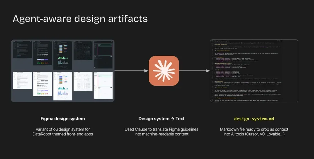
At DataRobot, the design system has been translated into machine-readable artifacts, together with Figma pointers, part specs, and interplay ideas expressed in markdown.
By encoding design requirements upstream, brokers can generate interfaces that stay constant, accessible, and on-brand with fewer guide evaluations that gradual innovation.
Turning design information into agent-aware artifacts ensures each generated software meets enterprise requirements for high quality and model consistency.
Designing for brokers as customers
One other shift: brokers themselves at the moment are customers. They work together with platforms, APIs, and workflows, typically extra instantly than people. This adjustments how suggestions, error dealing with, and collaboration are designed. Future-ready platforms won’t solely optimize for human-computer interplay, but additionally for human–agent collaboration.
Classes for design leaders
As boundaries blur, one reality stays: the laborious issues are nonetheless laborious. Agentic AI doesn’t erase these challenges — it makes them extra pressing. And it raises the stakes for design high quality. When anybody can spin up an app, consumer expertise, high quality, governance, and model alignment turn into the actual differentiators.
The enduring laborious issues
Perceive context: What unmet wants are actually being solved?
Design for constraints: Will it work with present architectures?
Tie tech to worth: Does this deal with issues that matter to the enterprise?
Ideas for navigating the shift
Construct programs, not simply merchandise: Deal with the foundations, constraints, and contexts that permit good experiences to emerge.
Train judgment: Use AI for velocity and execution, however depend on human experience and craft to determine what’s proper.
The blurring boundaries of the product triad.
Using the wave
Like Interstellar, what as soon as seemed like distant mountains are literally huge waves. Agentic AI isn’t on the horizon anymore—it’s right here. The enterprises that be taught to harness it won’t simply journey the wave. They may form what comes subsequent.
Study extra concerning the Agent Workforce Platform and the way DataRobot helps enterprises transfer from AI pilots to production-ready agentic programs.
After the final drop offered out in document time, the $400 MacBook Air is formally again, however possible not for lengthy. This 2020 M1 mannequin stays one of the widespread laptops Apple has ever made, and now it’s obtainable once more at a fraction of the standard value.
Powered by Apple’s M1 chip, this 13.3-inch MacBook Air delivers distinctive efficiency and battery life that may stretch as much as 18 hours on a single cost. It’s silent, quick, and nonetheless holds up superbly for on a regular basis use in 2025 from artistic work to binge-watching your favourite reveals.
What’s the take care of the MacBook Airs?
Apple M1 Chip with 8-core CPU and 8-core GPU for clean multitasking and video playback
512GB SSD and 8GB RAM for quick loading instances and beneficiant storage
13.3-inch Retina show with crisp, vivid shade for work or streaming
Fanless, light-weight design that runs cool and quiet
As much as 18 hours of battery life, relying on settings
Grade A refurbished situation — close to mint, with charger included
Contact ID and backlit Magic Keyboard for safe, snug use
The journey via superior academia, whether or not a Grasp’s thesis or a Ph.D. dissertation, begins not with the gathering of information, however with a meticulously crafted analysis proposal. For statisticians, this doc is way over a formality; it’s the final blueprint that demonstrates your mental rigor, material mastery, and, crucially, your potential to conduct a possible, sound, and impactful examine.
A successful statistics analysis proposal acts as your skilled constitution. It secures essential approval from supervisors, moral evaluate boards, and funding committees. In case you are grappling with find out how to write a analysis proposal in statistics, perceive this: your proposal should not merely define a subject, however current a flawless, built-in argument that your proposed investigation is critical, unique, and, above all, statistically viable.
This complete information is designed to empower you, breaking down the advanced course of into manageable, actionable phases, making certain your statistics analysis proposal achieves tutorial triumph.
The Core Distinction: Common vs. Statistics Analysis Proposals
Whereas each proposal shares basic sections (Introduction, Literature Evaluate, Methodology), the statistical proposal calls for absolute precision within the methodology part. Not like qualitative or basic quantitative research, your doc should:
Specify Hypotheses with Mathematical Readability: Clearly articulate the null (H0) and different (Ha) statistical speculation.
Justify Methodological Decisions: Clarify why a specific statistical mannequin (e.g., ARIMA, Logistic Regression, Combined-Results Modeling) is essentially the most acceptable software on your analysis query.
Display Energy and Precision: Embrace a proper pattern dimension calculation and energy evaluation, a non-negotiable a part of a very profitable analysis proposal.
Section 1: Constructing a Rock-Strong Basis (Conceptualization & Evaluate)
The preliminary part dictates the success of your total challenge. Dashing this stage usually results in basic flaws afterward.
Pinpointing Your Compelling Analysis Query
A fantastic statistical challenge begins with a testable query, not only a broad space of curiosity.
From Subject to Testable Speculation
Establish the Hole: What’s at present unknown or debated within the literature? As an illustration, “Does a selected new intervention X have an effect on consequence Y?”
Outline Variables: Clearly set up your dependent, unbiased, and potential confounding variables. Specify their measurement scales (nominal, ordinal, interval, ratio). This classification instantly informs the suitable statistical strategies in analysis you’ll use later.
Formulate the Statistical Speculation: Translate your analysis query into formal, quantifiable phrases.
Analysis Query Instance
Null Speculation (H0)
Various Speculation (Ha)
Does the brand new educating methodology (A) enhance check scores greater than the outdated methodology (B)?
μA=μB (There isn’t any distinction in imply check scores.)
μA>μB (Methodology A results in greater imply scores.)
The Strategic Literature Evaluate: An Argument, Not a Abstract
Your literature evaluate should do greater than checklist earlier research; it should construct a persuasive argument on your proposed work. It demonstrates your fluency with present analysis methodology statistics.
Critique and Synthesis: Focus on the statistical fashions utilized by others. Did they use ANOVA when a non-parametric check was required? Did they tackle multicollinearity of their regression?
Spotlight the Methodology Hole: Conclude the evaluate by clearly stating the place the present literature falls quick, justifying your distinctive statistical method. For instance, “Prior research utilized easy OLS regression; this statistics analysis proposal will pioneer using a hierarchical linear mannequin to account for the nested nature of the information, offering a extra strong inference.”
Section 2: The Core Elements of an Distinctive Proposal Construction
Each part of a analysis proposal should be completely aligned with the others. The stream from the Introduction to the Methodology should be seamless and logical.
Part 1: The Introduction and Significance (The Why)
This part is your alternative to seize the reader’s consideration and set up the significance of your work.
Drawback Assertion: A transparent, concise assertion of the issue your analysis addresses. Why ought to anybody care?
Goals and Aims: Use motion verbs (e.g., ‘to research’, ‘to mannequin’, ‘to check’). For instance, “The first goal is to check the statistical speculation that the likelihood of buyer churn is considerably predicted by the interplay of age and time on website utilizing a quantitative analysis proposal method.”
Significance: Element the theoretical and sensible implications. How will your findings contribute to statistical concept or real-world coverage?
Part 2: Methodology and Information Evaluation Plan (The Statistical Masterpiece)
That is essentially the most essential part for a statistics analysis proposal and requires the deepest dive. It should include adequate element for one more competent statistician to copy your examine.
Examine Design and Sampling Technique
Design Justification: Clearly specify the examine kind (e.g., experimental, quasi-experimental, observational, simulation). Justify why this design is essentially the most environment friendly and least biased technique to reply your analysis query.
Sampling: Element your inhabitants, pattern body, and sampling method (e.g., easy random, stratified, cluster). Clarify how this choice minimizes choice bias and maximizes generalizability.
The Statistical Precision: Pattern Dimension and Energy Evaluation
That is the place the proposal demonstrates feasibility and rigor.
The info evaluation plan should embrace the idea on your pattern dimension calculation (n). You have to state:
The specified stage of significance (α, sometimes 0.05).
The specified statistical energy (1−β, sometimes 0.80).
The impact dimension (d or η2) you intention to detect, primarily based on pilot information or prior literature.
Instance:
Pattern dimension was calculated utilizing G*Energy software program primarily based on detecting a average impact dimension (d=0.5) with 80% energy and a 5% significance stage. This yields a minimal requirement of n=64 per group for a two-sample t-test.
The Statistical Strategies in Analysis: Detailed Evaluation Plan
This subsection is the center of find out how to write a analysis proposal in statistics.
Descriptive Statistics: Checklist the abstract measures (Imply, SD, Median, IQR) and graphical shows (Histograms, Field Plots) you’ll use for preliminary information exploration.
Inferential Statistics: Explicitly title the first statistical check(s) for use to check your H0.
Instance (Time-Collection Information): “Major evaluation will make the most of an Autoregressive Built-in Transferring Common (ARIMA) mannequin to forecast the development, with the Ljung-Field Q-test used to test for autocorrelation within the residuals.”
Instance (Categorical Information): “A Binary Logistic Regression mannequin will likely be employed to estimate the chances of the binary consequence, controlling for 5 pre-specified covariates. Mannequin match will likely be assessed utilizing the Hosmer–Lemeshow check.”
Assumptions: For every methodology, checklist the important thing assumptions (e.g., normality, homoscedasticity, independence) and the diagnostic assessments you’ll carry out (e.g., Shapiro-Wilk for normality, Levene’s check for equality of variances).
Software program: Specify the statistical software program package deal (e.g., R, Python with NumPy/SciPy, SPSS) you’ll use.
Section 3: Feasibility, Ethics, and Anticipated Outcomes (The Logistics)
A robust proposal addresses not solely the mental problem but in addition the sensible realities of the challenge. That is essential for demonstrating that your quantitative analysis proposal is possible inside your timeline and assets.
Undertaking Timeline (Gantt Chart Advice)
An in depth, chapter-by-chapter or phase-by-phase timeline (usually offered as a Gantt chart) proves you might have a practical execution technique.
Section
Length
Key Deliverables (Statistical)
Literature Evaluate & Proposal Finalization
2 Months
Finalized Statistical Speculation and Information Administration Protocol.
Finalized Information Evaluation Plan report; Statistical Mannequin Output.
Thesis/Dissertation Writing
3 Months
Accomplished Draft.
Moral Issues and Information Administration
In statistical analysis, ethics primarily revolves round information.
Information Privateness: Element how you’ll anonymize or de-identify delicate information.
Storage and Safety: Describe the safe surroundings the place your uncooked information and analytical scripts will likely be saved, demonstrating compliance with information safety rules.
Limitations and Delimitations: Proving Statistical Consciousness
A trademark of an distinctive statistics analysis proposal is the sincere dialogue of limitations.
Limitations: Acknowledge potential threats to validity (e.g., pattern attrition, non-response bias, limitations of the chosen statistical strategies). Clarify your methods to mitigate these (e.g., a number of imputation for lacking information).
Delimitations: Clearly outline the boundaries of your examine (what you received’t examine), corresponding to limiting the examine inhabitants or excluding sure analytical methods to keep up focus.
The Flawless End: Last Evaluate for a Profitable Proposal Submission
Earlier than submitting your statistics analysis proposal, conduct a closing, rigorous evaluate.
Consistency Examine: Does the title precisely replicate the analysis query? Do the aims immediately align with the statistical speculation? Does the information evaluation plan logically comply with the methodology?
Readability and Movement: Is the proposal straightforward to learn? Have you ever averted overly dense paragraphs of textual content? Use bullet factors and tables (like those above) to reinforce readability and group.
Proofread for Technical Accuracy: A single misplaced statistical time period or formulation error can undermine your credibility. Make sure that the levels of freedom, p-values, and impact sizes are referenced appropriately in your dialogue of prior work.
Conclusion: Launching Your Distinctive Analysis Journey to Mastery!
Mastering find out how to write a analysis proposal in statistics is your first main step in direction of skilled and tutorial mastery. It forces you to suppose critically, methodologically, and, most significantly, statistically, earlier than you even interact with the information. By meticulously following this complete information—from formulating a transparent statistical speculation to detailing your information evaluation plan—you aren’t simply making a doc; you might be constructing the muse for a very impactful, rigorous, and in the end profitable analysis proposal.
Do I would like to gather my information earlier than submitting?
Usually, no. You want an in depth Information Evaluation Plan and proof of feasibility (e.g., entry to a pre-existing dataset or a transparent sampling technique and finances/timeline for assortment).
What’s the most crucial part for a statistics proposal?
The Methodology and Information Evaluation Plan. Reviewers must see an in depth, justified plan outlining your statistical fashions, assumptions, and energy calculation. Imprecise statements about utilizing “acceptable statistics” will result in rejection.
The place can I discover examples of robust methodology sections?
Many universities and analysis establishments present publicly accessible, profitable proposals. For an in depth information on find out how to construction and justify your method, you may seek advice from authoritative tutorial assets like this information on writing a analysis methodology part.