It’s difficult to generate the code for a whole consumer interface utilizing a Giant Language Mannequin (LLM). Person interfaces are complicated and their implementations typically encompass a number of, inter-related recordsdata that collectively specify the contents of every display, the navigation flows between the screens, and the information mannequin used all through the appliance. It’s difficult to craft a single immediate for an LLM that comprises sufficient element to generate a whole consumer interface, and even then the result’s continuously a single giant and obscure file that comprises the entire generated screens. On this paper, we introduce Athena, a prototype software era setting that demonstrates how using shared intermediate representations, together with an app storyboard, information mannequin, and GUI skeletons, might help a developer work with an LLM in an iterative style to craft a whole consumer interface. These intermediate representations additionally scaffold the LLM’s code era course of, producing organized and structured code in a number of recordsdata whereas limiting errors. We evaluated Athena with a consumer examine that discovered 75% of members most popular our prototype over a typical chatbot-style baseline for prototyping apps.
About two weeks in the past, we launched TensorFlow Likelihood (TFP), exhibiting find out how to create and pattern from distributions and put them to make use of in a Variational Autoencoder (VAE) that learns its prior. At the moment, we transfer on to a unique specimen within the VAE mannequin zoo: the Vector Quantised Variational Autoencoder (VQ-VAE) described in Neural Discrete Illustration Studying(Oord, Vinyals, and Kavukcuoglu 2017). This mannequin differs from most VAEs in that its approximate posterior isn’t steady, however discrete – therefore the “quantised” within the article’s title. We’ll rapidly take a look at what this implies, after which dive straight into the code, combining Keras layers, keen execution, and TFP.
Many phenomena are finest considered, and modeled, as discrete. This holds for phonemes and lexemes in language, higher-level buildings in pictures (suppose objects as a substitute of pixels),and duties that necessitate reasoning and planning.
The latent code utilized in most VAEs, nonetheless, is steady – often it’s a multivariate Gaussian. Steady-space VAEs have been discovered very profitable in reconstructing their enter, however usually they endure from one thing referred to as posterior collapse: The decoder is so highly effective that it could create real looking output given simply any enter. This implies there isn’t a incentive to study an expressive latent house.
In VQ-VAE, nonetheless, every enter pattern will get mapped deterministically to considered one of a set of embedding vectors. Collectively, these embedding vectors represent the prior for the latent house.
As such, an embedding vector comprises much more info than a imply and a variance, and thus, is far tougher to disregard by the decoder.
The query then is: The place is that magical hat, for us to tug out significant embeddings?
From the above conceptual description, we now have two inquiries to reply. First, by what mechanism can we assign enter samples (that went via the encoder) to applicable embedding vectors?
And second: How can we study embedding vectors that truly are helpful representations – that when fed to a decoder, will end in entities perceived as belonging to the identical species?
As regards task, a tensor emitted from the encoder is solely mapped to its nearest neighbor in embedding house, utilizing Euclidean distance. The embedding vectors are then up to date utilizing exponential transferring averages. As we’ll see quickly, because of this they’re really not being discovered utilizing gradient descent – a characteristic value stating as we don’t come throughout it every single day in deep studying.
Concretely, how then ought to the loss perform and coaching course of look? It will most likely best be seen in code.
The entire code for this instance, together with utilities for mannequin saving and picture visualization, is accessible on github as a part of the Keras examples. Order of presentation right here might differ from precise execution order for expository functions, so please to truly run the code take into account making use of the instance on github.
As in all our prior posts on VAEs, we use keen execution, which presupposes the TensorFlow implementation of Keras.
Along with the “standard” hyperparameters now we have in deep studying, the VQ-VAE infrastructure introduces a couple of model-specific ones. To begin with, the embedding house is of dimensionality variety of embedding vectors occasions embedding vector dimension:
# variety of embedding vectorsnum_codes<-64L# dimensionality of the embedding vectorscode_size<-16L
The latent house in our instance shall be of dimension one, that’s, now we have a single embedding vector representing the latent code for every enter pattern. This shall be advantageous for our dataset, nevertheless it must be famous that van den Oord et al. used far higher-dimensional latent areas on e.g. ImageNet and Cifar-10.
Encoder mannequin
The encoder makes use of convolutional layers to extract picture options. Its output is a three-D tensor of form batchsize * 1 * code_size.
activation<-"elu"# modularizing the code just a bit bitdefault_conv<-set_defaults(layer_conv_2d, listing(padding ="identical", activation =activation))
Now, every of those 16d vectors must be mapped to the embedding vector it’s closest to. This mapping is taken care of by one other mannequin: vector_quantizer.
Vector quantizer mannequin
That is how we’ll instantiate the vector quantizer:
This mannequin serves two functions: First, it acts as a retailer for the embedding vectors. Second, it matches encoder output to accessible embeddings.
Right here, the present state of embeddings is saved in codebook. ema_means and ema_count are for bookkeeping functions solely (be aware how they’re set to be non-trainable). We’ll see them in use shortly.
vector_quantizer_model<-perform(title=NULL, num_codes, code_size){keras_model_custom(title =title, perform(self){self$num_codes<-num_codesself$code_size<-code_sizeself$codebook<-tf$get_variable("codebook", form =c(num_codes, code_size), dtype =tf$float32)self$ema_count<-tf$get_variable( title ="ema_count", form =c(num_codes), initializer =tf$constant_initializer(0), trainable =FALSE)self$ema_means=tf$get_variable( title ="ema_means", initializer =self$codebook$initialized_value(), trainable =FALSE)perform(x, masks=NULL){# to be stuffed in shortly ...}})}
Along with the precise embeddings, in its name technique vector_quantizer holds the task logic.
First, we compute the Euclidean distance of every encoding to the vectors within the codebook (tf$norm).
We assign every encoding to the closest as by that distance embedding (tf$argmin) and one-hot-encode the assignments (tf$one_hot). Lastly, we isolate the corresponding vector by masking out all others and summing up what’s left over (multiplication adopted by tf$reduce_sum).
Concerning the axis argument used with many TensorFlow features, please take into accounts that in distinction to their k_* siblings, uncooked TensorFlow (tf$*) features anticipate axis numbering to be 0-based. We even have so as to add the L’s after the numbers to adapt to TensorFlow’s datatype necessities.
vector_quantizer_model<-perform(title=NULL, num_codes, code_size){keras_model_custom(title =title, perform(self){# right here now we have the above occasion fieldsperform(x, masks=NULL){# form: bs * 1 * num_codesdistances<-tf$norm(tf$expand_dims(x, axis =2L)-tf$reshape(self$codebook, c(1L, 1L, self$num_codes, self$code_size)), axis =3L)# bs * 1assignments<-tf$argmin(distances, axis =2L)# bs * 1 * num_codesone_hot_assignments<-tf$one_hot(assignments, depth =self$num_codes)# bs * 1 * code_sizenearest_codebook_entries<-tf$reduce_sum(tf$expand_dims(one_hot_assignments, -1L)*tf$reshape(self$codebook, c(1L, 1L, self$num_codes, self$code_size)), axis =2L)listing(nearest_codebook_entries, one_hot_assignments)}})}
Now that we’ve seen how the codes are saved, let’s add performance for updating them.
As we mentioned above, they don’t seem to be discovered by way of gradient descent. As an alternative, they’re exponential transferring averages, regularly up to date by no matter new “class member” they get assigned.
So here’s a perform update_ema that can deal with this.
first, maintain observe of the variety of at present assigned samples per code (updated_ema_count), and
second, compute and assign the present exponential transferring common (updated_ema_means).
moving_averages<-tf$python$coaching$moving_averages# decay to make use of in computing exponential transferring commondecay<-0.99update_ema<-perform(vector_quantizer,one_hot_assignments,codes,decay){updated_ema_count<-moving_averages$assign_moving_average(vector_quantizer$ema_count,tf$reduce_sum(one_hot_assignments, axis =c(0L, 1L)),decay, zero_debias =FALSE)updated_ema_means<-moving_averages$assign_moving_average(vector_quantizer$ema_means,# selects all assigned values (masking out the others) and sums them up over the batch# (shall be divided by rely later, so we get a mean)tf$reduce_sum(tf$expand_dims(codes, 2L)*tf$expand_dims(one_hot_assignments, 3L), axis =c(0L, 1L)),decay, zero_debias =FALSE)updated_ema_count<-updated_ema_count+1e-5updated_ema_means<-updated_ema_means/tf$expand_dims(updated_ema_count, axis =-1L)tf$assign(vector_quantizer$codebook, updated_ema_means)}
Earlier than we take a look at the coaching loop, let’s rapidly full the scene including within the final actor, the decoder.
Decoder mannequin
The decoder is fairly customary, performing a collection of deconvolutions and eventually, returning a likelihood for every picture pixel.
Now we’re prepared to coach. One factor we haven’t actually talked about but is the associated fee perform: Given the variations in structure (in comparison with customary VAEs), will the losses nonetheless look as anticipated (the standard add-up of reconstruction loss and KL divergence)?
We’ll see that in a second.
Coaching loop
Right here’s the optimizer we’ll use. Losses shall be calculated inline.
The coaching loop, as standard, is a loop over epochs, the place every iteration is a loop over batches obtained from the dataset.
For every batch, now we have a ahead move, recorded by a gradientTape, based mostly on which we calculate the loss.
The tape will then decide the gradients of all trainable weights all through the mannequin, and the optimizer will use these gradients to replace the weights.
To date, all of this conforms to a scheme we’ve oftentimes seen earlier than. One level to notice although: On this identical loop, we additionally name update_ema to recalculate the transferring averages, as these usually are not operated on throughout backprop.
Right here is the important performance:
num_epochs<-20for(epochinseq_len(num_epochs)){iter<-make_iterator_one_shot(train_dataset)until_out_of_range({x<-iterator_get_next(iter)with(tf$GradientTape(persistent =TRUE)%as%tape, {# do ahead move# calculate losses})encoder_gradients<-tape$gradient(loss, encoder$variables)decoder_gradients<-tape$gradient(loss, decoder$variables)optimizer$apply_gradients(purrr::transpose(listing(encoder_gradients, encoder$variables)), global_step =tf$prepare$get_or_create_global_step())optimizer$apply_gradients(purrr::transpose(listing(decoder_gradients, decoder$variables)), global_step =tf$prepare$get_or_create_global_step())update_ema(vector_quantizer,one_hot_assignments,codes,decay)# periodically show some generated pictures# see code on github # visualize_images("kuzushiji", epoch, reconstructed_images, random_images)})}
Now, for the precise motion. Contained in the context of the gradient tape, we first decide which encoded enter pattern will get assigned to which embedding vector.
Now, for this task operation there isn’t a gradient. As an alternative what we will do is move the gradients from decoder enter straight via to encoder output.
Right here tf$stop_gradient exempts nearest_codebook_entries from the chain of gradients, so encoder and decoder are linked by codes:
In sum, backprop will deal with the decoder’s in addition to the encoder’s weights, whereas the latent embeddings are up to date utilizing transferring averages, as we’ve seen already.
Now we’re able to sort out the losses. There are three parts:
First, the reconstruction loss, which is simply the log likelihood of the particular enter beneath the distribution discovered by the decoder.
Second, now we have the dedication loss, outlined because the imply squared deviation of the encoded enter samples from the closest neighbors they’ve been assigned to: We wish the community to “commit” to a concise set of latent codes!
Lastly, now we have the standard KL diverge to a previous. As, a priori, all assignments are equally possible, this part of the loss is fixed and might oftentimes be distributed of. We’re including it right here primarily for illustrative functions.
And right here we go. This time, we will’t have the second “morphing view” one usually likes to show with VAEs (there simply isn’t any second latent house). As an alternative, the 2 pictures beneath are (1) letters generated from random enter and (2) reconstructed precise letters, every saved after coaching for 9 epochs.
Left: letters generated from random enter. Proper: reconstructed enter letters.
Two issues soar to the attention: First, the generated letters are considerably sharper than their continuous-prior counterparts (from the earlier submit). And second, would you’ve been capable of inform the random picture from the reconstruction picture?
At this level, we’ve hopefully satisfied you of the ability and effectiveness of this discrete-latents method.
Nevertheless, you would possibly secretly have hoped we’d apply this to extra advanced knowledge, similar to the weather of speech we talked about within the introduction, or higher-resolution pictures as present in ImageNet.
The reality is that there’s a steady tradeoff between the variety of new and thrilling methods we will present, and the time we will spend on iterations to efficiently apply these methods to advanced datasets. Ultimately it’s you, our readers, who will put these methods to significant use on related, actual world knowledge.
Clanuwat, Tarin, Mikel Bober-Irizar, Asanobu Kitamoto, Alex Lamb, Kazuaki Yamamoto, and David Ha. 2018. “Deep Studying for Classical Japanese Literature.” December 3, 2018. https://arxiv.org/abs/cs.CV/1812.01718.
Oord, Aaron van den, Oriol Vinyals, and Koray Kavukcuoglu. 2017. “Neural Discrete Illustration Studying.”CoRR abs/1711.00937. http://arxiv.org/abs/1711.00937.
With the Apple Watch Extremely 2 in your wrist, you may go wherever you need, and also you’ll discover your method again residence, whether or not you’re climbing, mountaineering, or simply out for a stroll, because the watch will know your location always and present you the correct map. Even higher, with built-in mobile, you don’t even must have your cellphone on you.
Again when this mannequin got here out, we reviewed it and gave it a 4-star ranking, appreciating the intense display screen, nice working system, and simply how nice it was for monitoring sports activities and exercises. This mannequin comes with 36 hours of battery life throughout regular use, so it’s going to be nice throughout any out of doors journey you need This gadget comes with a ton of options, together with correct location monitoring, superior well being metrics, customized exercises, in addition to automated fall detection, emergency SOS, and important signal monitoring. If something occurs, your watch has your again.
There’s a newer mannequin out, however aside from higher battery life and satellite tv for pc connectivity, it’s not all that completely different than this one. And also you gained’t get it for wherever close to this low-cost. So seize the Apple Watch Extremely 2 for $499 earlier than the spring sale ends.
The Antennae Galaxies pictured merging within the constellation Corvus. (Picture credit score: Greg Meyer)
Astrophotographer Greg Meyer took purpose on the constellation Corvus to seize an imposing view of the Antennae Galaxies, whose as soon as spiral varieties have been rendered chaotic as they merge right into a single elliptical monster of a galaxy.
The deep area picture captures a fleeting second in a titanic battle that has lasted a whole lot of thousands and thousands of years, because the gravitational affect of the galaxies NGC 4038 and NGC 4039 pulls at each other to create chaos on a very cosmic scale.
“I’ve a Sky-Watcher Esprit 120 [telescope] with a focal size of 840mm, which is a bit brief for many galaxies, this being galaxy season now,” Meyer informed Area.com in an electronic mail. “So every time I see an image of a galaxy, I see whether it is inside attain for me by checking Astrobin for images taken with the identical scope. And since that is such a cool picture of two galaxies, with an incredible backstory, I needed to go for it.”
Article continues beneath
Meyer’s shot reveals the orange-yellow cores of the dueling galaxies glowing in a maelstrom of interstellar mud, gasoline and stars, from which a pair of sweeping “tidal tails” created from elongated spiral arms attain out for light-years on both facet. The sweeping buildings bear a placing resemblance to the sensory organs sported by members of the insect world, which finally granted them the nickname of the Antennae Galaxies.
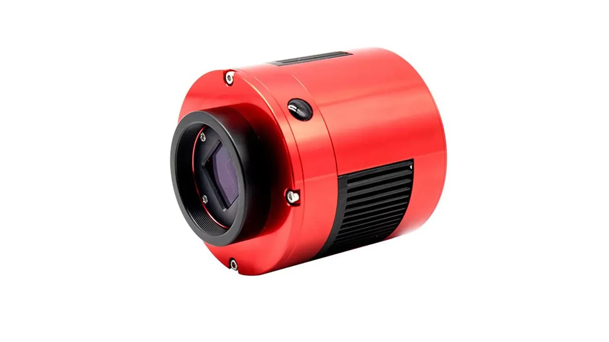
ZWO ASI533MC Professional
(Picture credit score: Amazon)
The ZWO ASI533MC Professional digital camera is one of the best devoted astro digital camera on the market, in our opinion. It options zero amp glow, 80% quantum effectivity and a 20FPS body charge. It additionally contains a 9MP sensor and you’ll take a look at our ZWO ASI533MC Professional evaluate for a extra in-depth look.
The cosmic tug of battle has triggered an outburst of star formation, which has led to the creation of “tremendous star clusters” within the huge antenna-like arms, in line with NASA. 90% of those goliath clusters are more likely to disperse because the galaxies merge and settle, whereas others will persevere as globular clusters.
Meyer devoted slightly below 21 hours of statement time accumulating gentle from the distant galaxies utilizing a collection of astronomy filters as they glowed within the skies over the Starfront Observatory in Rockwood, Texas. The sunshine information was then compiled and edited utilizing Adobe Photoshop and Lightroom in live performance with the astrophotography software program PixInsight.
Breaking area information, the most recent updates on rocket launches, skywatching occasions and extra!
Editor’s Word: If you need to share your astrophotography with Area.com’s readers, then please ship your picture(s), feedback, and your identify and placement to spacephotos@area.com.
Statistics is a necessary topic that helps college students perceive knowledge, patterns, and traits. Many college students search for statistics undertaking concepts for school college students to finish tutorial assignments and develop analytical abilities. Engaged on statistics tasks permits college students to use theoretical ideas to actual life issues. As an alternative of solely studying formulation, college students get the chance to gather knowledge, analysis outcomes and draw significant conclusions.
Statistics tasks are generally utilized in fields equivalent to arithmetic, economics, social sciences and knowledge science. These tasks assist college students enhance their analysis abilities and sensible expertise in statistical evaluation. On this information, we are going to discover artistic and sensible statistics undertaking concepts for school college students that may allow you to construct a powerful tutorial undertaking.
Why Statistics Tasks Are Vital
Statistics tasks play an necessary function in creating analytical and analysis abilities amongst college students. By engaged on actual knowledge, college students learn the way statistical ideas are utilized in sensible conditions.
Enhance Analytical Expertise
Statistics tasks assist college students analyze actual world knowledge and determine patterns, traits and relationships.
Develop Analysis Skills
College students discover ways to conduct surveys, gather knowledge and interpret statistical outcomes.
Improve Downside-Fixing Expertise
Information evaluation encourages important considering and logical reasoning.
Actual World Functions
Statistics is extensively utilized in enterprise, economics, healthcare and expertise industries.
20+ Statistics Mission Concepts for Faculty College students
Beneath are some attention-grabbing statistics undertaking concepts together with easy examples.
1. Research Habits vs Educational Efficiency
This undertaking research the connection between research habits and tutorial outcomes.
Instance
2 hours
60%
4 hours
75%
6 hours
88%
College students can discover whether or not longer research hours enhance tutorial efficiency.
2. Social Media Utilization Amongst Faculty College students
Analyze how social media utilization impacts research time and productiveness.
Instance
1 hour
4 hours
2 hours
3 hours
4 hours
2 hours
3. Affect of Sleep on Educational Efficiency
This undertaking research how sleep period impacts pupil efficiency.
Instance
5 hours
60%
7 hours
75%
8+ hours
82%
4. On-line Buying Habits of College students
Instance
Survey of fifty faculty college students:
As soon as a month
35%
2–3 instances a month
40%
Weekly
25%
College students can analyze the commonest purchasing frequency.
5. Health and Bodily Exercise Statistics
Instance
Survey knowledge from college students:
0–1 hour
Excessive
2–3 hours
Medium
4+ hours
Low
This knowledge highlights the connection between train and stress.
6. Film Choice Evaluation
Instance
Survey outcomes:
Motion
30%
Comedy
25%
Drama
20%
Sci-Fi
15%
Different
10%
College students can current this knowledge with a pie chart.
7. Meals Consumption Patterns
Instance
Information collected from college students:
Quick Meals
40%
Dwelling Meals
35%
Wholesome Food plan
25%
This knowledge might be displayed with bar charts.
8. Web Utilization Patterns
Instance
Survey results:
Educational Research
3 hours
Social Media
2 hours
Leisure
1.5 hours
College students can evaluate tutorial and leisure use.
9. Transportation Decisions of College students
Instance
Transportation survey:
Bus
40%
Bike
30%
Automobile
20%
Strolling
10%
This info can reveal the commonest mode of transportation.
10. Price range Administration Amongst College students
Instance
Month-to-month spending knowledge:
Meals
$120
Leisure
$60
Transport
$40
Research Supplies
$30
College students can analyze their spending priorities.
11. Gaming Habits Amongst College students
Instance
Gaming survey:
0–1 hour
30%
1–3 hours
45%
3+ hours
25%
College students can assess whether or not gaming impacts research time.
12. Music Listening Preferences
Instance
Survey knowledge:
Pop
35%
Hip-Hop
25%
Rock
20%
Classical
10%
Different
10%
This knowledge reveals college students music preferences.
13. Display screen Time Statistics
Instance
Every day display screen time:
Smartphone
4 hours
Laptop computer
3 hours
Pill
1 hour
College students can analyze the affect of display screen time on productiveness.
14. Stress Ranges Throughout Exams
Instance
Scholar stress survey:
1–2 hours
Excessive
3–4 hours
Medium
5+ hours
Low
College students can consider the connection between research habits and stress.
15. Library Utilization Patterns
Instance
Library go to data:
College students can study how library utilization impacts tutorial efficiency.
16. Attendance vs Educational Efficiency
Instance
Attendance knowledge:
This knowledge reveals the connection between attendance and grades.
17. On-line Studying Effectiveness
Instance
Survey outcomes:
College students can assess the effectiveness of on-line studying.
18 Half Time Jobs Amongst College students
Instance
Work hours knowledge:
0 hours
3.6
10 hours
3.3
20 hours
3.0
College students can analyze the steadiness between work and research.
19 Smartphone Model Preferences
Instance
Model reputation survey:
Apple
35%
Samsung
30%
Xiaomi
20%
Different
15%
College students can research shopper preferences.
20 Weekend Actions of College students
Instance
Weekend exercise survey:
Finding out
30%
Socializing
40%
Hobbies
20%
Relaxation
10%
College students can analyze patterns in pupil existence.
21 Research Time vs Examination Outcomes
Instance
Research hours knowledge:
2 hours
60%
4 hours
75%
6 hours
88%
College students can visualize this knowledge with a scatter plot.
Instruments Used for Statistics Tasks
College students can use quite a lot of instruments to take a look at statistics and see how knowledge is distributed.
Frequent instruments embrace:
These instruments assist college students set up knowledge, carry out calculations and create graphs for higher evaluation.
Suggestions for Selecting a Good Statistics Mission
Select a Related Subject
Select a topic that has to do with precise life or college life.
Use Dependable Information
Correct knowledge helps produce significant outcomes.
Give attention to Clear Evaluation
Clarify statistical findings clearly and logically.
Use Graphs and Charts
Visible representations make knowledge simpler to know.
Conclusion
Statistics tasks assist faculty college students develop necessary analysis and analytical abilities. By working with actual world knowledge and exploring sensible matters, college students can higher perceive statistical ideas and their functions.
The undertaking concepts listed on this information present a powerful place to begin for tutorial analysis. Whether or not analyzing social media habits, research habits or life-style patterns, statistics tasks permit college students to use theoretical data to actual life conditions.
With the fitting subject correct knowledge assortment and correct evaluation college students can create significant tasks that enhance their tutorial data and put together them for careers in knowledge pushed fields.
Continuously Requested Questions
What are statistics undertaking concepts?
Statistics undertaking concepts are case research that contain amassing, learning and deciphering knowledge.
Why are statistics tasks necessary?
They assist college students develop analytical considering, analysis capabilities and knowledge interpretation abilities.
How do you select an excellent statistics undertaking subject?
Select a subject that’s partaking, appropriate and has simply obtainable knowledge.
Which instruments are generally used for statistics tasks?
Instruments like Excel, Google Sheets and R programming are generally used for statistical evaluation.
In in the present day’s quickly evolving job market, technical experience alone will not be sufficient. Employers more and more search well-rounded candidates who mix robust technical abilities with important human abilities—resembling communication, collaboration, adaptability, and emotional intelligence.
This want is much more important in gentle of the rise of synthetic intelligence (AI) and automation, that are reworking workplaces and reshaping job roles.
Human abilities: The important edge in an AI-driven world
Whereas AI excels at automating routine duties and analyzing huge quantities of information, it can not replicate uniquely human skills like empathy, creativity, important considering, compassion, and interpersonal communication. These human abilities, or comfortable abilities, allow professionals to navigate advanced social dynamics, construct belief, and lead groups successfully—capabilities which might be indispensable in any office. Employers acknowledge that candidates who reveal each technical and human abilities are higher outfitted to adapt to alter, resolve issues innovatively, and collaborate throughout numerous groups.
Skilled abilities programs to enhance technical coaching
To deal with this very important want, Cisco Networking Academy presents a group of Skilled Abilities programs designed to enhance technical coaching with interpersonal skill-building. These programs empower learners to develop the human abilities that AI can not change, getting ready them to thrive within the trendy office. Cisco Networking Academy has continued to broaden our assortment, now providing 10+ Skilled Abilities programs.
Core Abilities: Quick, sensible programs specializing in important interpersonal abilities within the office which might be important for achievement throughout industries – resembling communication, teamwork, problem-solving, and emotional intelligence. Learners apply these abilities in programs resembling Partaking Stakeholders for Success and Creating Compelling Studies, which embody interactive workouts in skilled communication and relationship administration.
Entrepreneurship: A 3-course sequence cultivating entrepreneurial considering and a solution-oriented mindset to navigate challenges creatively – from discovery to launching and managing a enterprise enterprise. Learners discover industry-standard frameworks such because the enterprise mode canvas, lean mannequin canvas, and SWOT evaluation. Key subjects embody finance and accounting, advertising methods, pitch deck growth, and networking abilities important for startup success.
English for IT: Programs to construct English language proficiency, tailor-made for IT professionals to boost communication in world tech environments. These programs cowl important terminology and situations throughout key sectors together with cybersecurity, tech assist, software program growth, DevOps, Machine Studying, and extra. Programs begin from the fundamentals (A2 proficiency) all the best way up by way of B2 proficiency to arrange for the English for IT B2/GSE 59-75 certification examination.
Profession Abilities: Entry profession preparation and job search assets and instruments to assist learners transitioning into the workforce. Acquire sensible steerage on crafting an expert resume, interview prep, and constructing a social media presence–together with an optimized LinkedIn profile. Via our partnership with Certainly, you possibly can entry a curated profession hub that includes job alternatives aligned together with your Cisco Networking Academy abilities and certifications.
As AI and automation advance, the significance of human abilities grows. Skilled Abilities programs are designed to assist learners achieve a aggressive edge by mastering these irreplaceable skills. Our versatile, on-line, self-paced programs are particularly well-suited for college kids, early-in-career, and profession changers. As well as, academic organizations can supply instructor-led variations of those programs to boost their program choices and develop well-rounded, aggressive job candidates.
Enroll without spending a dime
Benefit from Cisco Networking Academy’s Skilled Abilities programs. They’re out there for free of charge, and it’s straightforward to get began and be taught at your personal tempo. These programs not solely complement your technical experience but in addition make it easier to construct the interpersonal abilities employers worth most. You’ll additionally earn Cisco-verified digital badges to showcase your achievements.
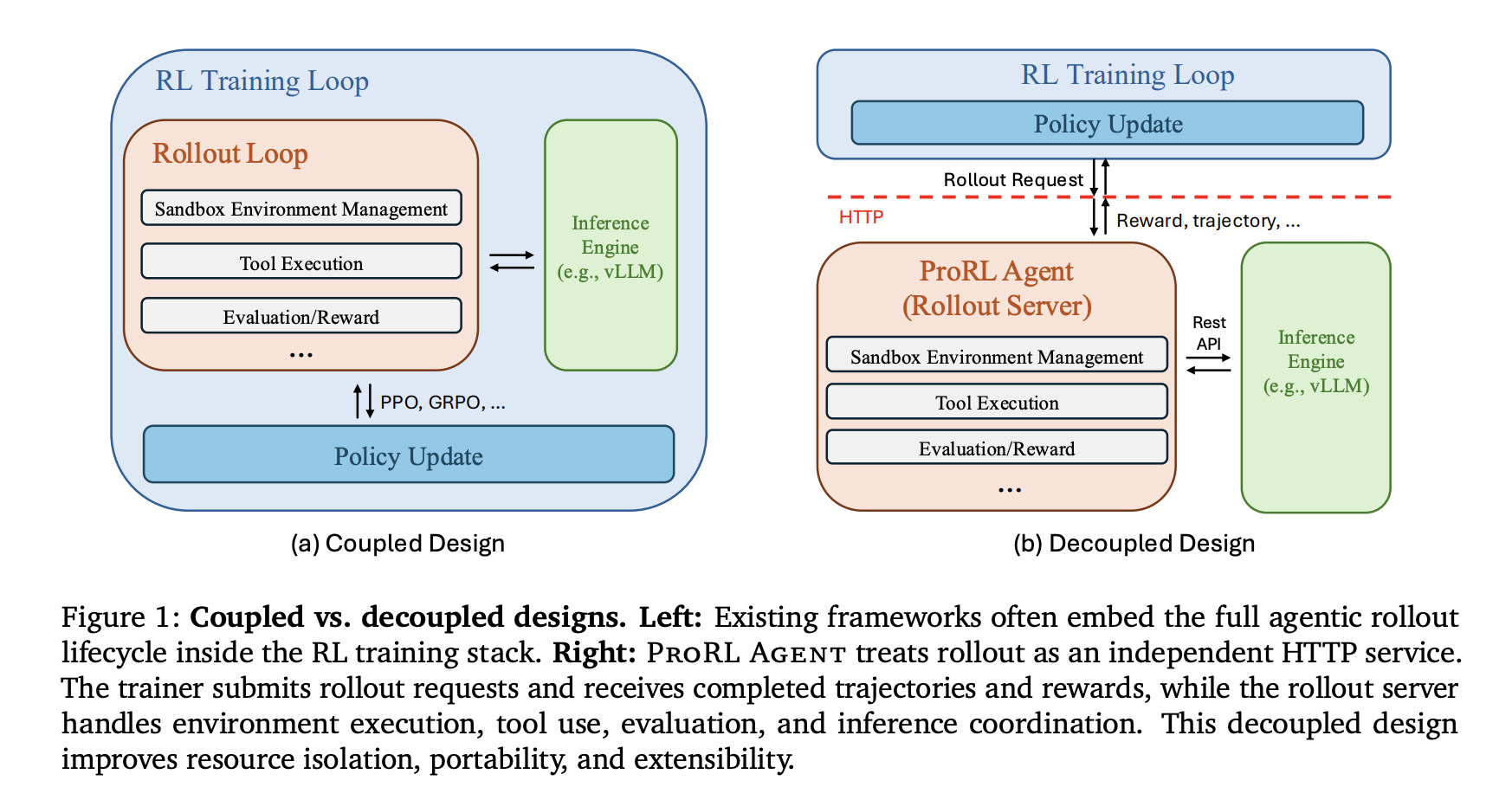
NVIDIA researchers launched ProRL AGENT, a scalable infrastructure designed for reinforcement studying (RL) coaching of multi-turn LLM brokers. By adopting a ‘Rollout-as-a-Service’ philosophy, the system decouples agentic rollout orchestration from the coaching loop. This architectural shift addresses the inherent useful resource conflicts between I/O-intensive setting interactions and GPU-intensive coverage updates that at present bottleneck agent improvement.
The Core Downside: Tight Coupling
Multi-turn agent duties contain interacting with exterior environments, corresponding to code repositories or working techniques, through iterative software use. Many present frameworks—together with SkyRL, VeRL-Device, Agent Lightning, rLLM, and GEM—embed rollout management straight throughout the coaching course of.
This tight coupling results in two major limitations:
Conflicting System Necessities: Rollouts are I/O-bound, requiring sandbox creation, long-lived software classes, and asynchronous coordination. Coaching is GPU-intensive, centered on ahead/backward passes and gradient synchronization. Operating each in a single course of causes interference and reduces {hardware} effectivity.
Upkeep Obstacles: Embedding rollout logic within the coach makes it troublesome emigrate to completely different coaching backends or assist new runtime environments with out re-implementing the execution pipeline.
https://arxiv.org/pdf/2603.18815
System Design: Rollout-as-a-Service
ProRL AGENT operates as a standalone HTTP service that manages the total rollout lifecycle. The RL coach interacts with the server solely via an API, remaining agnostic to the underlying rollout infrastructure.
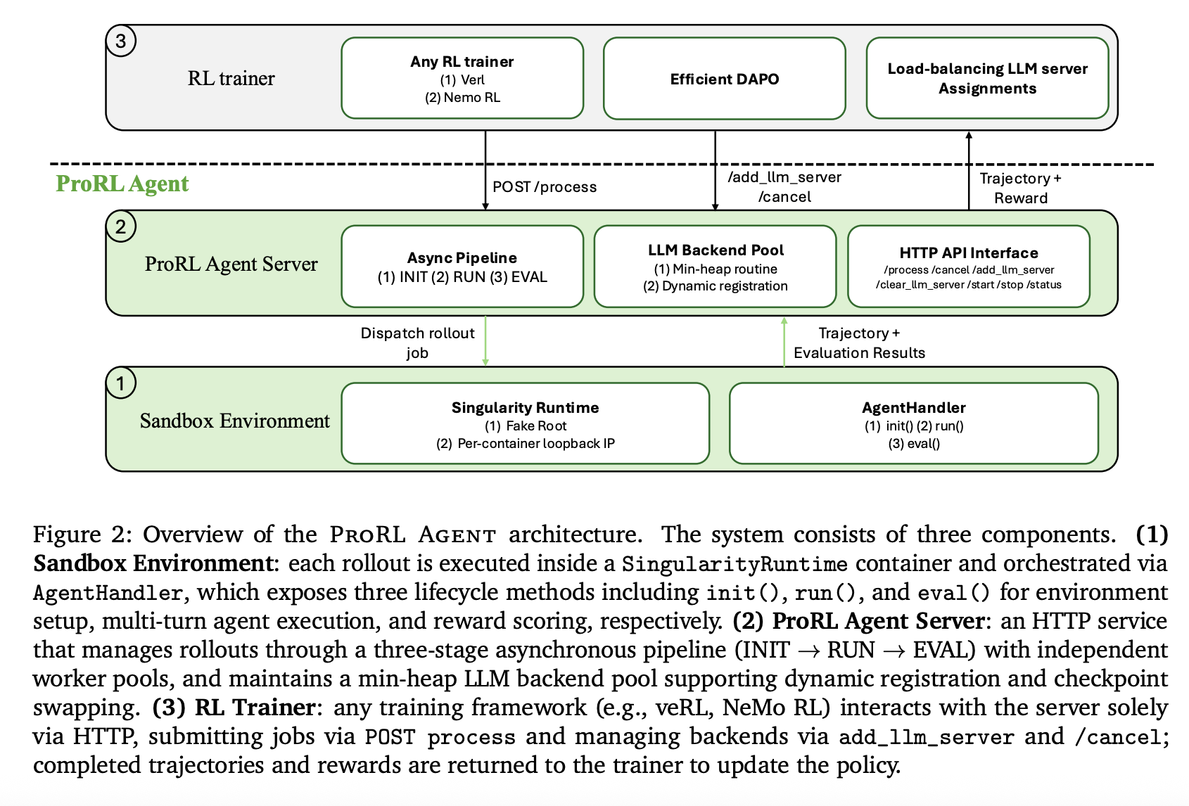
Three-Stage Asynchronous Pipeline
To maximise throughput, the server orchestrates rollouts via an asynchronous three-stage ‘meeting line’:
INIT: Initialization employees spin up sandbox containers and configure instruments.
RUN: Rollout employees drive the multi-turn agent loop and accumulate trajectories.
EVAL: Analysis employees rating outcomes towards floor reality to provide reward indicators.
By assigning every stage to an impartial employee pool, ProRL AGENT permits phases to overlap throughout completely different jobs, stopping gradual evaluations (corresponding to full check suite executions) from stalling the rollout course of.
https://arxiv.org/pdf/2603.18815
HPC-Appropriate Sandboxing and Optimized Instruments
ProRL AGENT makes use of Singularity for its sandbox infrastructure. In contrast to Docker-based platforms, Singularity permits rootless execution, which is required for deployment on shared HPC clusters managed by Slurm.
The system contains a number of optimizations to scale back software execution latency, which frequently dominates complete rollout time:
Environment friendly Bash: Replaces tmux-based terminal multiplexing with a ptyprocess-based direct pseudo-terminal, lowering shell command latency from 0.78s to 0.42s.
Direct IPython API: Connects to persistent kernels through an in-process API as a substitute of community gateways, eradicating networking overhead.
Unix Area Sockets (UDS): Replaces TCP loopback for communication between the agent and the execution server contained in the container to shave off further latency.
Superior Options for Scalable RL
The infrastructure introduces mechanisms to enhance coaching stability and {hardware} utilization:
Load Balancing and Prefix Cache Reuse
The server manages a pool of LLM inference backends (e.g., vLLM) utilizing a min-heap keyed by project counts. When a job is assigned, all subsequent calls inside that job are routed to the identical backend. This technique maximizes prefix cache reuse, lowering inference time throughout a number of agent turns.
Token-in/Token-out Communication
To eradicate re-tokenization drift—the place the token sequence generated throughout rollout differs from what’s used throughout coaching—ProRL AGENT makes use of token IDs because the canonical illustration all through the complete course of. Log-probabilities and IDs are propagated unchanged from the inference backend to the coach.
Optimized DAPO Implementation
The system helps Dynamic Sampling Coverage Optimization (DAPO), which filters out ‘non-informative’ prompts that yield uniform rewards. ProRL AGENT makes use of an asynchronous replenishment mechanism to take care of most throughput, terminating redundant lively jobs early as soon as the goal variety of informative prompts is reached.
Experimental Outcomes on SWE-Bench Verified
The system was validated utilizing Qwen3 fashions throughout a number of scales. ProRL AGENT persistently improved efficiency in comparison with reproduced baselines.
Mannequin Scale
Reproduced Baseline
ProRL Agent (RL)
Qwen3-4B
14.8
21.2
Qwen3-8B
9.6
18.0
Qwen3-14B
15.4 (reproduced baseline)
23.6
Notice: The reported prior consequence for SkyRL-Agent-14B-v0 was 21.6.
Along with software program engineering, the system demonstrated generality in STEM, Math, and Code domains, displaying regular reward progress throughout RL coaching. Scalability checks confirmed that rollout throughput will increase near-linearly as compute nodes are added.
Key Takeaways
Architectural Decoupling: ProRL Agent treats the total agentic rollout lifecycle—together with setting initialization, software execution, and reward scoring—as an impartial HTTP service, separating I/O-intensive duties from GPU-intensive coverage coaching.
Vital Efficiency Beneficial properties: This infrastructure enabled the Qwen3-8B mannequin to just about double its efficiency on the SWE-Bench Verified benchmark (from 9.6% to 18.0%), whereas the Qwen3-14B mannequin improved from 15.4% to 23.6%.
System Latency Reductions: Focused optimizations, corresponding to changing tmux with ptyprocess for shell execution, diminished motion latency from 0.78s to 0.42s, contributing to near-linear throughput scaling throughout compute nodes.
Elimination of Tokenization Drift: The framework makes use of a token-in/token-out communication pipeline, making certain that the precise token IDs generated throughout rollout are handed to the coach with out the chance of lossy re-tokenization.
HPC-Native Deployment: By utilizing Singularity as a substitute of Docker, ProRL Agent helps rootless execution and native Slurm integration, permitting large-scale agent coaching on shared high-performance computing clusters.
One UI 9 rumors proceed, as a report claims Samsung is allegedly testing Accessibility settings updates for customers.
Such settings may assist customers spotlight or increase textual content a lot simpler than earlier than, alongside upgraded mouse and keyboard updates to make actions simpler.
One UI 9 rumors first acquired underway a few weeks in the past, however they had been minimal, as solely UI refinements/modifications had been acknowledged.
Samsung is already pushing forward with One UI 9, and one report claims it is trying to weave in an replace to its accessibility options.
One other dive into Samsung’s alleged early One UI 9 code by tipster AssembleDebug and Android Authority sheds gentle on what may come to go. The tipster’s findings reportedly unearthed a number of strings of code that time towards an improve for Galaxy telephones’ Accessibility settings. Nevertheless, upon deeper inspection, AssembleDebug claims to have discovered particular “Textual content Highlight” updates.
This function is not new, very like lots of them, as Android Authority additionally notes, however what we’re listening to is the rumor that this might convey a faucet function for “increasing and highlighting textual content.” Moreover, customers may be capable to customise the dimensions and coloration if that’s required.
Article continues under
Android Central’s Take
Samsung’s rolled out Accessibility updates earlier than, and it is all within the title of showing simple to method for all customers. From text-to-speech to bigger textual content for these with imaginative and prescient points, it is all in good religion. These are small (alleged) updates, however hopefully they’re going to have large impacts once we get to see them for actual, if that is to be believed.
Samsung may additionally embrace “faucet indicators” to enlarge textual content and spotlight it in a “separate window.” There are additionally two updates to Galaxy’s keyboard and mouse Accessibility options. The tipster alleges one replace may enable customers to maneuver their related mouse with their keyboard, in addition to a “fine-tuning” choice for cursor velocity. The opposite issues a “bodily keyboard shortcut.” This might let customers flip Accessibility settings on or off with out going into their cellphone’s settings.
AssembleDebug talked about a change to the swiping or single-tap choice. Now, it appears One UI 9 will place this on the “prime stage” of the Interplay menu.
Ease of use
(Picture credit score: Nicholas Sutrich / Android Central)
It is nonetheless pretty early. One UI 9 shall be primarily based on Android 17, which has gotten off to a quick begin in 2026. Google even rolled out Beta 3 late this week. Proper now, what’s acquired us occupied are One UI 9 rumors, which acquired underway earlier in March. A report claimed that Samsung has began internally testing the following main OS launch. This might debut first on the corporate’s subsequent wave of foldables. It is not the strangest factor that would occur, as we have seen this earlier than.
Android Central’s Take
I do suppose the funniest factor that would’ve occurred is the looks of One UI 9 leaks, and Galaxy S25 house owners nonetheless do not have v8.5. It is actually early to begin fascinated by One UI 9, particularly since these leaks are nonetheless fairly minimal. Are we big modifications? I am unsure. One UI 8.5 was fairly substantial, so it’d look to relax on any heavy-handed modifications.
What was a bit of odd is that this information surfaced at a time when the vast majority of Samsung’s telephones, just like the S25 and S24, do not have One UI 8.5 but. Little or no was talked about about One UI 9’s upgrades. It was alluded that Samsung may’ve been testing Fast Settings refinements and shifting Parental Controls into its personal devoted web page.
Get the most recent information from Android Central, your trusted companion on the planet of Android
We might earn income from the merchandise out there on this web page and take part in affiliate packages. Be taught extra ›
Signal Up For Items 🛍️
Product information, evaluations, and must-have offers.
Amazon’s Large Spring Sale is reside proper now with deep reductions throughout house items — we’re speaking 52% off mattresses, 50% off vacuums, 44% off bedding units, and critical cuts on Dyson, KitchenAid, Shark, Casper, LEVOIT, and extra. Whether or not you’re upgrading your kitchen, refreshing your bed room, or lastly tackling the storage, this is among the finest house offers occasions of the yr. We dug by way of each class to search out those truly value shopping for.
Dyson V8 Plus Cordless Vacuum $329.99 (was $539.99)
The Dyson V8 Plus is 39% off proper now — $210 off one in every of Dyson’s best-selling cordless vacuums. It handles each onerous flooring and carpet, delivers as much as 40 minutes of runtime, and contains the Detangling Motorbar head that cuts by way of pet hair with out wrapping. When you’ve been ready for a Dyson to drop to an inexpensive value, that is the second.
Shark Pet Cordless Stick Vacuum $149.00 (was $299.99)
This Shark is down a full 50% — the largest proportion low cost in the whole sale. It’s a cordless stick vacuum constructed particularly for pet house owners, with a self-cleaning brushroll that removes pet hair robotically. At $149, it’s distinctive worth for anybody coping with fur on flooring and furnishings.
CAROTE 26-Piece Nonstick Pots and Pans Set $129.99 (was $219.99)
A 26-piece nonstick cookware set for $130 is genuinely sturdy worth — that is 41% off. CAROTE’s granite-coated pans are PFOA-free, dishwasher protected, and induction appropriate. Getting pots, pans, lids, and utensils in a single bundle at this value is the form of kitchen refresh that often prices twice as a lot.
Vacuum and ground care offers
Among the deepest reductions within the sale land on vacuums and ground care — Dyson, Shark, and Bissell are all right here with cuts as much as 50%. Whether or not you want a cordless stick vac, a wet-dry ground washer, or a transportable spot cleaner, there are strong choices at each value level.
Air air purifier and humidifier offers
LEVOIT, Coway, and AIRDOCTOR are all discounted — protecting small bedrooms as much as giant open-plan areas. Spring allergy season is the suitable time to consider indoor air high quality.
Kitchen equipment offers
That is the place the sale shines for house cooks. Breville, KitchenAid, Ninja, Cuisinart, Instantaneous Pot, and Keurig are all discounted — from espresso machines and stand mixers down to non-public blenders and air fryers. A few of these are the bottom costs of the yr on their respective fashions.
Past home equipment, there are sturdy offers on precise cookware — nonstick pan units, forged iron instruments, meals storage, and kitchen equipment. The KitchenAid dish rack at 49% off is a standout, and the Caraway ceramic pan is a pleasant choose for these wanting a cleaner cooking floor.
Mattress and topper offers
Main reductions from Casper, Tempur-Pedic, ZINUS, EGOHOME, and extra — mattresses in each measurement, firmness, and value vary. Reminiscence foam toppers are additionally steeply discounted if you wish to prolong the lifetime of what you have already got. Among the price range choices right here hit over 50% off.
Bedding, décor, and bathtub offers
From natural cotton sheet units to blackout curtains, satin pillowcases, throw blankets, and bathtub towels — there’s a variety of bed room and loo upgrades right here at sturdy reductions. Sheet units underneath $30 and curtains underneath $15 are uncommon outdoors of a sale like this.
Space rug offers
Washable space rugs are having a second, and the Large Spring Sale has a number of choices with as much as 36% off. Large rugs hardly ever get this low-cost — particularly machine-washable ones that may truly maintain up long-term.
Furnishings offers
Workplace chairs, mattress frames, sofas, and bookshelves — the furnishings part spans a variety, with strong cuts on name-brand items from La-Z-Boy, HON, Sauder, Zinus, and Avenco. The La-Z-Boy government chairs particularly are at sturdy costs.
Storage and group offers
Clear bins, over-toilet racks, wall cabinets, shoe storage, and closet organizers — if spring cleansing is on the checklist, this part has what you want. Vtopmart, ClearSpace, BAYKA, and YFXCVSL all have strong offers with 18–41% off.
Backyard, garden, and out of doors offers
Spring is the suitable time to put money into the yard, and the Large Spring Sale has offers on grills, grass seed, develop lights, water filtration, and instruments. Whether or not you’re organising a container backyard, tackling a full garden renovation, or simply restocking on pest management, there are strong choices right here.
Dwelling cleansing and family necessities offers
Inventory-up financial savings on the belongings you truly use each week — dishwasher pods, laundry detergent, disinfecting wipes, rest room bowl cleaners, and oral care. Not glamorous, however reductions on consumables add up shortly over time.
What’s it about spherical numbers that compels us to pause and replicate? We have a good time 20-year faculty reunions, 25-year marriage ceremony anniversaries, fiftieth birthdays and different comparable milestones. I don’t know the reply however the Stata YouTube Channel lately handed a number of milestones – greater than 1500 subscribers, over 50,000 video views and it was launched six months in the past. We felt the necessity for a small celebration to mark the event, and I assumed that I might provide you with a short replace.
I might inform you about re-recording the unique 24 movies with a bigger font to make them simpler to learn. I might inform you concerning the {hardware} and software program that we use to document them together with our experiments with varied condenser and dynamic microphones. I might share quotes from a number of the good messages we’ve obtained. However I feel it will be extra enjoyable to speak about….you!
YouTube collects information concerning the variety of views every video receives in addition to abstract information about who, what, when, the place, and the way you might be watching them. There isn’t any have to be involved about your privateness; there aren’t any private identifiers of any type related to these information. However the abstract information are fascinating, and I assumed it is perhaps enjoyable to share a number of the information with you.
Who’s watching?
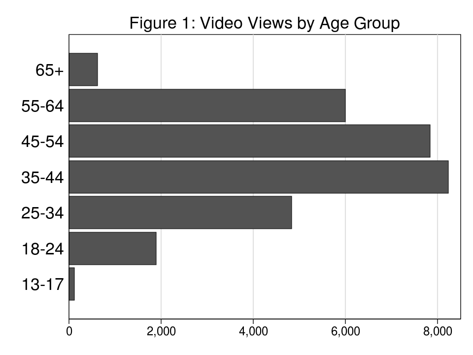
Determine 1 exhibits the age distribution of Stata YouTube Channel viewers. When you have ever attended a Stata Convention, you’ll not be shocked by this graph…till you discover the age group on the backside. I might not have guessed that 13-17 12 months olds are watching our movies. Maybe they noticed Stata within the film “Moneyball” with Brad Pitt and wished to study extra. Or possibly they had been influenced by the newest trend craze sweeping the youth of the world.
What are you watching?
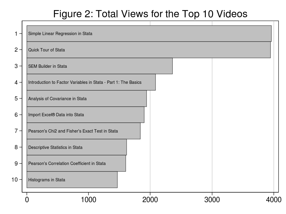
We’ve posted greater than 50 movies over a variety of matters. Determine 2 exhibits the whole variety of views for the ten hottest movies. The extra in style of the ten are about broad matters. These broader movies are principally older and have thus had time to build up extra views.
Even so, these movies obtain extra views per day presently than do the particular subject movies which were posted extra lately. This helps my perception that Stata YouTube Channel viewers are usually comparatively new Stata customers who need to find out about common matters, and which means extra generic movies sooner or later. So that you and your two post-docs will simply should learn the handbook if you wish to discover ways to match uneven energy ARCH fashions with outer-product gradient commonplace errors.
When are you watching?
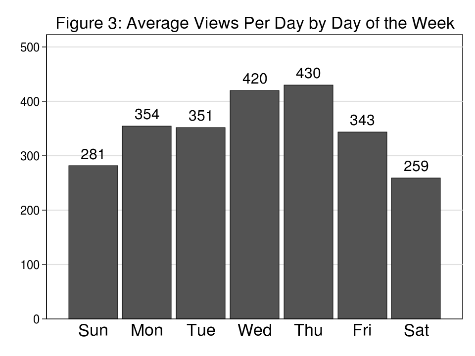
We often submit new movies on Tuesday mornings which could lead you to consider that the height viewing day would even be Tuesday. Determine 3, nevertheless, exhibits us that the common variety of views per day (vpd) is greater on Wednesdays at 420 vpd and actually peaks on Thursdays at 430 vpd earlier than declining Friday via Sunday.
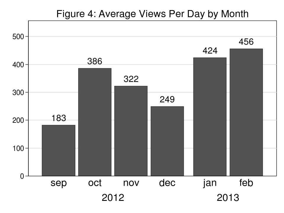
Determine 4 additionally exhibits us that late September might have been not the most effective time to launch the Stata YouTube Channel. Our early momentum in September and October slowed throughout the November and December vacation seasons. We had been, nevertheless, happy to see that 49 of you spent New Years Eve watching our movies. Maybe subsequent 12 months we’ll put together one thing extra festive only for you!
The place are you watching?
What do the Czech Republic, Pakistan, Uganda, Madagascar, the UK, the Bahamas, the US, Montenegro, and Italy have in frequent? Appropriate! They’re all nations during which you might be watching our movies. They’re additionally places depicted in considered one of my favourite motion movies however I’ll go away that to the trivia buffs. I feel essentially the most thrilling info that we present in our information is that the Stata YouTube Channel is being considered in 164 nations!
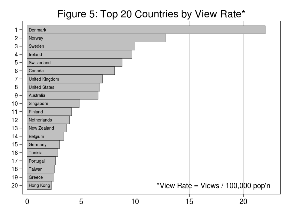
You may not be shocked to study that roughly half of the folks watching the movies stay in the US, the UK, or Canada. The outcomes could also be surprising after we take into account the “view charge” outlined because the variety of views per 100,000 residents. Determine 5 exhibits the highest 20 nations ranked by view charge for nations with a minimum of 4 million residents. Denmark had the very best view charge which was practically twice the speed of Norway which had the second highest view charge. The view charge in Denmark was greater than thrice the speed within the US and the UK.
How are you watching?
You may suppose that I might have something to report about “how” you might be watching the movies, but it surely seems that 5.2% of you might be watching on cellular units. Maybe this explains the 13-17 12 months outdated demographic or the 49 folks watching on New Yr’s Eve. Or possibly we’re serving to you cross the time within the dentist workplace ready room.
Last ideas
Six months isn’t a lot of a milestone. We Stata folks will use any excuse to interrupt out the cake and ice cream. Even so, the Stata YouTube Channel started as an experiment and sometimes experiments don’t work out as we want. This experiment has exceeded our expectations and, consequently, we’ve began taking requests for movies on our Fb web page and we’ll be including extra movies each week. So thanks for watching and keep tuned!
Now if you’ll excuse me, I’m going to get some cake and ice cream.


