Picture by Creator
# Introduction
AI has moved from merely chatting with giant language fashions (LLMs) to giving them legs and arms, which permits them to carry out actions within the digital world. These are sometimes known as Python AI brokers — autonomous software program packages powered by LLMs that may understand their surroundings, make selections, use exterior instruments (like APIs or code execution), and take actions to realize particular targets with out fixed human intervention.
When you have been eager to experiment with constructing your personal AI agent however felt weighed down by complicated frameworks, you might be in the correct place. In the present day, we’re going to take a look at smolagents, a strong but extremely easy library developed by Hugging Face.
By the top of this text, you’ll perceive what makes smolagents distinctive, and extra importantly, you should have a functioning code agent that may fetch dwell information from the web. Let’s discover the implementation.
# Understanding Code Brokers
Earlier than we begin coding, let’s perceive the idea. An agent is basically an LLM geared up with instruments. You give the mannequin a aim (like “get the present climate in London”), and it decides which instruments to make use of to realize that aim.
What makes the Hugging Face brokers within the smolagents library particular is their method to reasoning. In contrast to many frameworks that generate JSON or textual content to resolve which instrument to make use of, smolagents brokers are code brokers. This implies they write Python code snippets to chain collectively their instruments and logic.
That is highly effective as a result of code is exact. It’s the most pure strategy to categorical complicated directions like loops, conditionals, and information manipulation. As a substitute of the LLM guessing methods to mix instruments, it merely writes the Python script to do it. As an open-source agent framework, smolagents is clear, light-weight, and ideal for studying the basics.
// Conditions
To comply with alongside, you will have:
- Python data. Try to be snug with variables, capabilities, and pip installs.
- A Hugging Face token. Since we’re utilizing the Hugging Face ecosystem, we are going to use their free inference API. You will get a token by signing up at huggingface.co and visiting your settings.
- A Google account is non-compulsory. If you do not need to put in something domestically, you’ll be able to run this code in a Google Colab pocket book.
# Setting Up Your Surroundings
Let’s get our workspace prepared. Open your terminal or a brand new Colab pocket book and set up the library.
mkdir demo-project
cd demo-project
Subsequent, let’s arrange our safety token. It’s best to retailer this as an surroundings variable. In case you are utilizing Google Colab, you need to use the secrets and techniques tab within the left panel so as to add HF_TOKEN after which entry it by way of userdata.get('HF_TOKEN').
# Constructing Your First Agent: The Climate Fetcher
For our first undertaking, we are going to construct an agent that may fetch climate information for a given metropolis. To do that, the agent wants a instrument. A instrument is only a perform that the LLM can name. We’ll use a free, public API known as wttr.in, which gives climate information in JSON format.
// Putting in and Setting Up
Create a digital surroundings:
A digital surroundings isolates your undertaking’s dependencies out of your system. Now, let’s activate the digital surroundings.
Home windows:
macOS/Linux:
You will note (env) in your terminal when energetic.
Set up the required packages:
pip set up smolagents requests python-dotenv
We’re putting in smolagents, Hugging Face’s light-weight agent framework for constructing AI brokers with tool-use capabilities; requests, the HTTP library for making API calls; and python-dotenv, which is able to load surroundings variables from a .env file.
That’s it — all with only one command. This simplicity is a core a part of the smolagents philosophy.
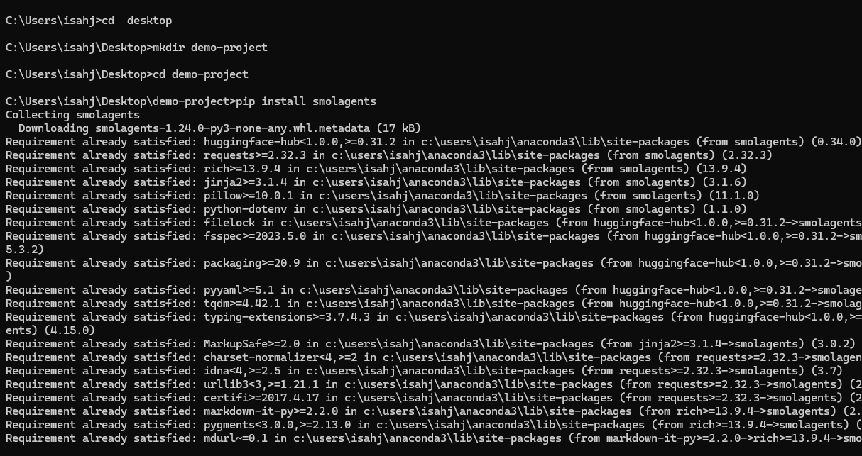
Determine 1: Putting in smolagents
// Setting Up Your API Token
Create a .env file in your undertaking root and paste this code. Please change the placeholder together with your precise token:
HF_TOKEN=your_huggingface_token_here
Get your token from huggingface.co/settings/tokens. Your undertaking construction ought to appear to be this:
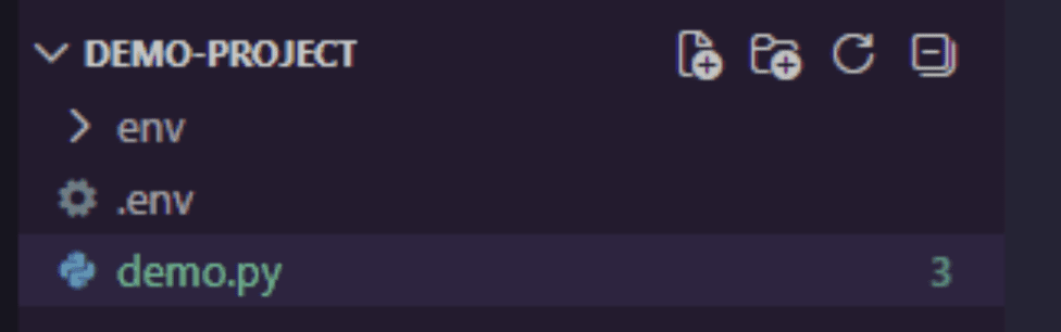
Determine 2: Undertaking construction
// Importing Libraries
Open your demo.py file and paste the next code:
import requests
import os
from smolagents import instrument, CodeAgent, InferenceClientModel
requests: For making HTTP calls to the climate APIos: To securely learn surroundings variablessmolagents: Hugging Face’s light-weight agent framework offering:@instrument: A decorator to outline agent-callable capabilities.CodeAgent: An agent that writes and executes Python code.InferenceClientModel: Connects to Hugging Face’s hosted LLMs.
In smolagents, defining a instrument is simple. We’ll create a perform that takes a metropolis title as enter and returns the climate situation. Add the next code to your demo.py file:
@instrument
def get_weather(metropolis: str) -> str:
    """
    Returns the present climate forecast for a specified metropolis.
    Args:
        metropolis: The title of the town to get the climate for.
    """
    # Utilizing wttr.wherein is a beautiful free climate service
    response = requests.get(f"https://wttr.in/{metropolis}?format=%C+%t")
    if response.status_code == 200:
        # The response is obvious textual content like "Partly cloudy +15°C"
        return f"The climate in {metropolis} is: {response.textual content.strip()}"
    else:
        return "Sorry, I could not fetch the climate information."
Let’s break this down:
- We import the
instrumentdecorator from smolagents. This decorator transforms our common Python perform right into a instrument that the agent can perceive and use. - The docstring (
""" ... """) within theget_weatherperform is vital. The agent reads this description to know what the instrument does and methods to use it. - Contained in the perform, we make a easy HTTP request to wttr.in, a free climate service that returns plain-text forecasts.
- Sort hints (
metropolis: str) inform the agent what inputs to offer.
It is a excellent instance of instrument calling in motion. We’re giving the agent a brand new functionality.
// Configuring the LLM
hf_token = os.getenv("HF_TOKEN")
if hf_token is None:
    increase ValueError("Please set the HF_TOKEN surroundings variable")

mannequin = InferenceClientModel(
    model_id="Qwen/Qwen2.5-Coder-32B-Instruct",
    token=hf_token
)
The agent wants a mind — a big language mannequin (LLM) that may cause about duties. Right here we use:
Qwen2.5-Coder-32B-Instruct: A strong code-focused mannequin hosted on Hugging FaceHF_TOKEN: Your Hugging Face API token, saved in a.envfile for safety
Now, we have to create the agent itself.
agent = CodeAgent(
    instruments=[get_weather],
    mannequin=mannequin,
    add_base_tools=False
)
CodeAgent is a particular agent sort that:
- Writes Python code to unravel issues
- Executes that code in a sandboxed surroundings
- Can chain a number of instrument calls collectively
Right here, we’re instantiating a CodeAgent. We move it a listing containing our get_weather instrument and the mannequin object. The add_base_tools=False argument tells it to not embrace any default instruments, preserving our agent easy for now.
// Operating the Agent
That is the thrilling half. Let’s give our agent a activity. Run the agent with a particular immediate:
response = agent.run(
    "Are you able to inform me the climate in Paris and in addition in Tokyo?"
)
print(response)
Whenever you name agent.run(), the agent:
- Reads your immediate.
- Causes about what instruments it wants.
- Generates code that calls
get_weather("Paris")andget_weather("Tokyo"). - Executes the code and returns the outcomes.
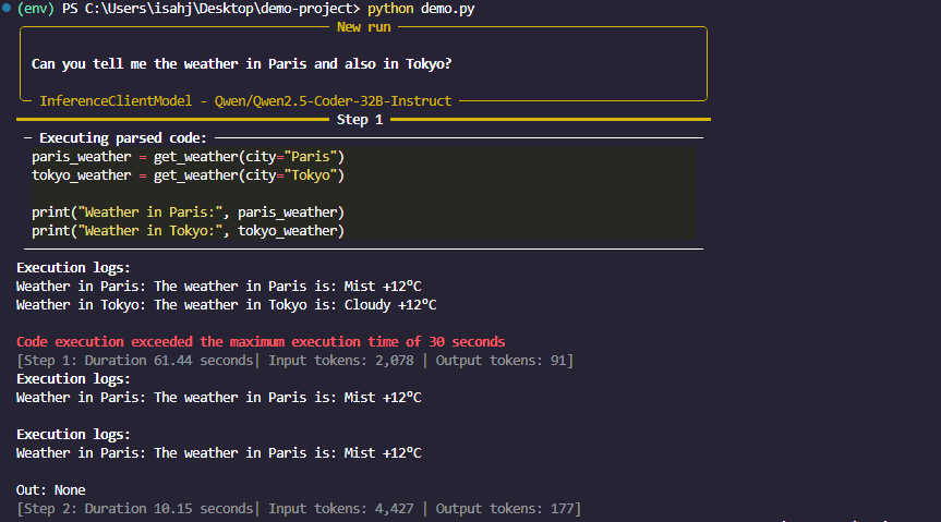
Determine 3: smolagents response
Whenever you run this code, you’ll witness the magic of a Hugging Face agent. The agent receives your request. It sees that it has a instrument known as get_weather. It then writes a small Python script in its “thoughts” (utilizing the LLM) that appears one thing like this:
That is what the agent thinks, not code you write.
weather_paris = get_weather(metropolis="Paris")
weather_tokyo = get_weather(metropolis="Tokyo")
final_answer(f"Right here is the climate: {weather_paris} and {weather_tokyo}")
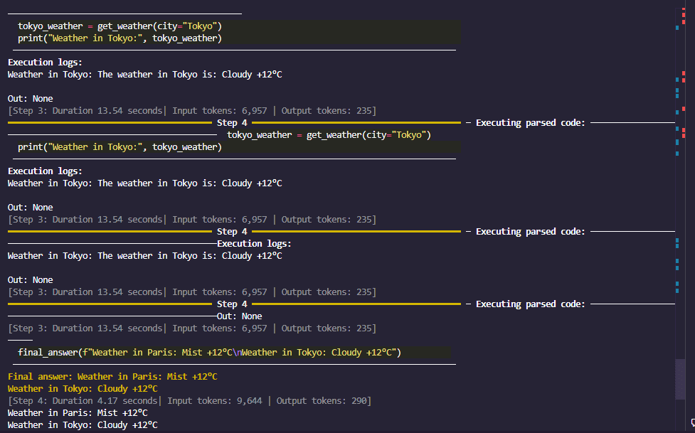
Determine 4: smolagents remaining response
It executes this code, fetches the info, and returns a pleasant reply. You’ve got simply constructed a code agent that may browse the net by way of APIs.
// How It Works Behind the Scenes
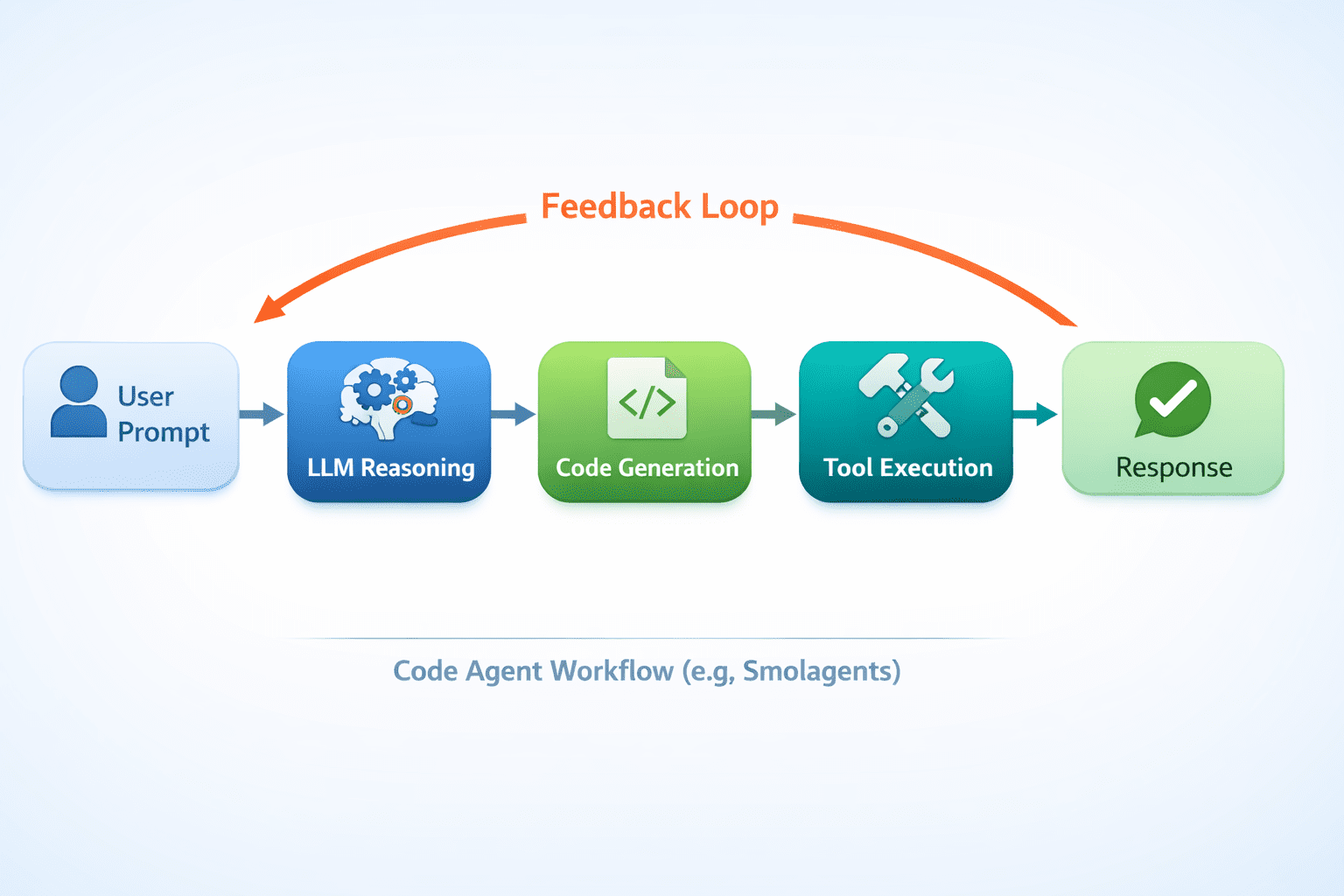
Determine 5: The interior workings of an AI code agent
// Taking It Additional: Including Extra Instruments
The facility of brokers grows with their toolkit. What if we needed to save lots of the climate report back to a file? We are able to create one other instrument.
@instrument
def save_to_file(content material: str, filename: str = "weather_report.txt") -> str:
    """
    Saves the supplied textual content content material to a file.
    Args:
        content material: The textual content content material to save lots of.
        filename: The title of the file to save lots of to (default: weather_report.txt).
    """
    with open(filename, "w") as f:
        f.write(content material)
    return f"Content material efficiently saved to {filename}"

# Re-initialize the agent with each instruments
agent = CodeAgent(
    instruments=[get_weather, save_to_file],
    mannequin=mannequin,
)
agent.run("Get the climate for London and save the report back to a file known as london_weather.txt")
Now, your agent can fetch information and work together together with your native file system. This mix of expertise is what makes Python AI brokers so versatile.
# Conclusion
In just some minutes and with fewer than 20 strains of core logic, you have got constructed a practical AI agent. We’ve got seen how smolagents simplifies the method of making code brokers that write and execute Python to unravel issues.
The fantastic thing about this open-source agent framework is that it removes the boilerplate, permitting you to concentrate on the enjoyable half: constructing the instruments and defining the duties. You’re not simply chatting with an AI; you might be collaborating with one that may act. That is only the start. Now you can discover giving your agent entry to the web by way of search APIs, hook it as much as a database, or let it management an online browser.
// References and Studying Assets
Shittu Olumide is a software program engineer and technical author enthusiastic about leveraging cutting-edge applied sciences to craft compelling narratives, with a eager eye for element and a knack for simplifying complicated ideas. You can even discover Shittu on Twitter.