Google has added two new service tiers to the Gemini API that allow enterprise builders to regulate the price and reliability of AI inference relying on how time-sensitive a given workload is.
Whereas the price of coaching massive language fashions for synthetic intelligence has been a priority prior to now, the main focus of consideration is more and more transferring to inferencing, or the value of utilizing these fashions.
The brand new tiers, referred to as Flex Inference and Precedence Inference, handle an issue that has grown extra acute as enterprises transfer past easy AI chatbots into advanced, multi-step agentic workflows, the corporate mentioned in a weblog put up printed Thursday.
In a separate announcement on the identical day, Google additionally launched Gemma 4, the most recent era of its open mannequin household for builders preferring to run fashions domestically fairly than through a paid API, describing it as its most succesful open launch so far.
The brand new API service tiers are meant to simplify life for builders of agentic methods involving background duties that don’t require immediate responses and interactive, user-facing options the place reliability is vital. Till now, supporting each workload varieties meant sustaining separate architectures: normal synchronous serving for real-time requests and the asynchronous Batch API for much less time-sensitive jobs.
“Flex and Precedence assist to bridge this hole,” the put up mentioned. “Now you can route background jobs to Flex and interactive jobs to Precedence, each utilizing normal synchronous endpoints.”
The 2 tiers function by means of a single synchronous interface, with precedence set through a service_tier parameter within the API request.
Decrease value vs larger availability
Flex Inference is priced at 50% of the usual Gemini API price, however affords lowered reliability and better latency. I is suited to background CRM updates, large-scale analysis simulations, and agentic workflows “the place the mannequin ‘browses’ or ‘thinks’ within the background,” Google mentioned. It’s out there to all paid-tier customers for GenerateContent and Interactions API requests.
For enterprise platform groups, the sensible worth is that background AI workloads corresponding to information enrichment, doc processing, and automatic reporting could be run at materially decrease value with no separate asynchronous structure, and with out the necessity to handle enter/output information or ballot for job completion.
Precedence Inference provides requests the very best processing precedence on Google’s infrastructure, “even throughout peak load,” the put up said.
Nonetheless, as soon as a buyer’s site visitors exceeds their Precedence allocation, overflow requests whereas not outright rejected are routinely routed to the Normal tier as an alternative.
“This retains your utility on-line and helps to make sure enterprise continuity,” Google mentioned, including that the API response will point out which tier dealt with every request, giving builders visibility into each efficiency and billing. Precedence Inference is offered to Tier 2 and Tier 3 paid tasks.
However the downgrade mechanism raises issues for regulated industries, in accordance ot Greyhound Analysis Chief Analyst Sanchit Vir Gogia.
“Two an identical requests, submitted underneath completely different system circumstances, can expertise completely different latency, completely different prioritisation, and probably completely different outcomes,” he mentioned. “In isolation, this appears like a efficiency problem. In follow, it turns into an consequence integrity problem.”
For banking, insurance coverage, and healthcare, he mentioned, that variability raises direct questions round equity, explainability, and auditability. “Sleek degradation, with out full transparency and governance, isn’t resilience,” Gogia mentioned. “It’s ambiguity launched into the system at scale.”
What it means for enterprise AI technique
The brand new tiers are a part of a broader business shift towards tiered inference pricing that Gogia mentioned displays constrained AI infrastructure fairly than purely business innovation.
“Tiered inference pricing is the clearest sign but that AI compute is transitioning right into a utility mannequin,” he mentioned, “however with out the maturity, transparency, or standardisation that enterprises usually affiliate with utilities.” The underlying driver, he mentioned, is structural shortage — energy availability, specialised {hardware}, and information centre capability — and tiering is how suppliers are managing allocation underneath these constraints.
For CIOs and procurement groups, vendor contracts can now not stay generic, Gogia mentioned. “They need to explicitly outline service tiers, define downgrade circumstances, implement efficiency ensures, and set up mechanisms for value management and auditability.”
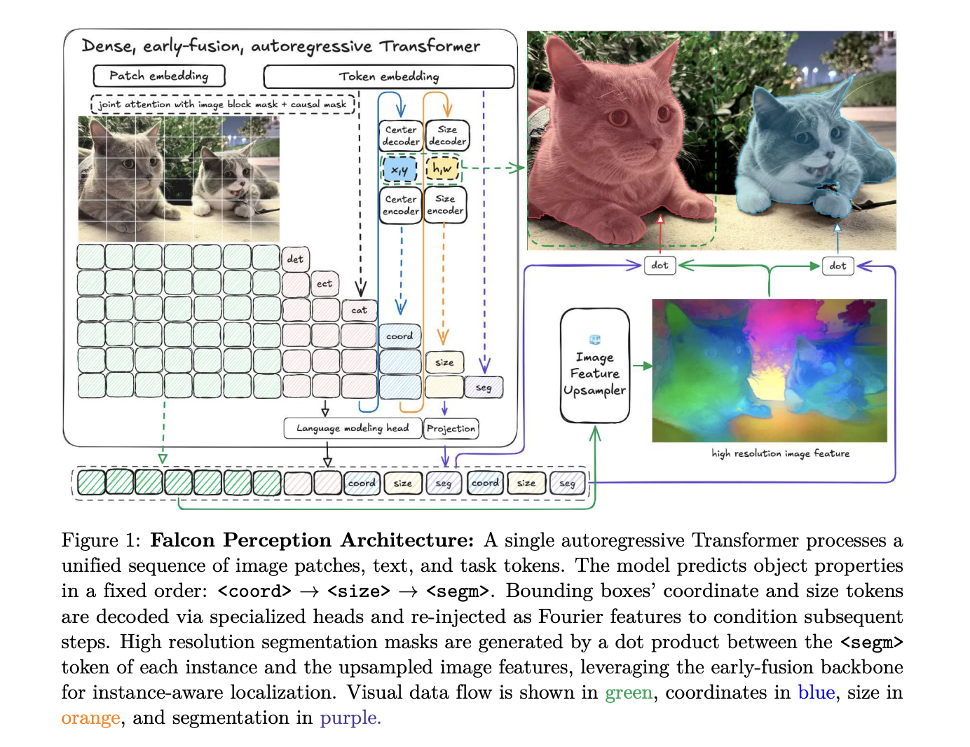
Within the present panorama of pc imaginative and prescient, the usual working process entails a modular ‘Lego-brick’ strategy: a pre-trained imaginative and prescient encoder for function extraction paired with a separate decoder for activity prediction. Whereas efficient, this architectural separation complicates scaling and bottlenecks the interplay between language and imaginative and prescient.
The Expertise Innovation Institute (TII) analysis crew is difficult this paradigm with Falcon Notion, a 600M-parameter unified dense Transformer. By processing picture patches and textual content tokens in a shared parameter area from the very first layer, TII analysis crew has developed an early-fusion stack that handles notion and activity modeling with excessive effectivity.
https://arxiv.org/pdf/2603.27365
The Structure: A Single Stack for Each Modality
The core design of Falcon Notion is constructed on the speculation {that a} single Transformer can concurrently study visible representations and carry out task-specific technology.
Hybrid Consideration and GGROPE
Not like customary language fashions that use strict causal masking, Falcon Notion employs a hybrid consideration technique. Picture tokens attend to one another bidirectionally to construct a world visible context, whereas textual content and activity tokens attend to all previous tokens (causal masking) to allow autoregressive prediction.
To take care of 2D spatial relationships in a flattened sequence, the analysis crew makes use of 3D Rotary Positional Embeddings. This decomposes the pinnacle dimension right into a sequential part and a spatial part utilizing Golden Gate ROPE (GGROPE). GGROPE permits consideration heads to take care of relative positions alongside arbitrary angles, making the mannequin sturdy to rotation and side ratio variations.
Minimalist Sequence Logic
The essential architectural sequence follows a Chain-of-Notion format:
[Image] [Text] ... .
This ensures that the mannequin resolves spatial ambiguity (place and measurement) as a conditioning sign earlier than producing the ultimate segmentation masks.
Engineering for Scale: Muon, FlexAttention, and Raster Ordering
TII analysis crew launched a number of optimizations to stabilize coaching and maximize GPU utilization for these heterogeneous sequences.
Muon Optimization: The analysis crew report that using the Muon optimizer for specialised heads (coordinates, measurement, and segmentation) led to decrease coaching losses and improved efficiency on benchmarks in comparison with customary AdamW.
FlexAttention and Sequence Packing: To course of photos at native resolutions with out losing compute on padding, the mannequin makes use of a scatter-and-pack technique. Legitimate patches are packed into fixed-length blocks, and FlexAttention is used to limit self-attention inside every picture pattern’s boundaries.
Raster Ordering: When a number of objects are current, Falcon Notion predicts them in raster order (top-to-bottom, left-to-right). This was discovered to converge quicker and produce decrease coordinate loss than random or size-based ordering.
The Coaching Recipe: Distillation to 685GT
The mannequin makes use of multi-teacher distillation for initialization, distilling data from DINOv3 (ViT-H) for native options and SigLIP2 (So400m) for language-aligned options. Following initialization, the mannequin undergoes a three-stage notion coaching pipeline totaling roughly 685 Gigatokens (GT):
In-Context Itemizing (450 GT): Studying to ‘listing’ the scene stock to construct international context.
Job Alignment (225 GT): Transitioning to independent-query duties utilizing Question Masking to make sure the mannequin grounds every question solely on the picture.
Lengthy-Context Finetuning (10 GT): Brief adaptation for excessive density, growing the masks restrict to 600 per expression.
Throughout these levels, the task-specific serialization is used:
expr1expr2.
The and tokens drive the mannequin to decide to a binary determination on an object’s existence earlier than localization.
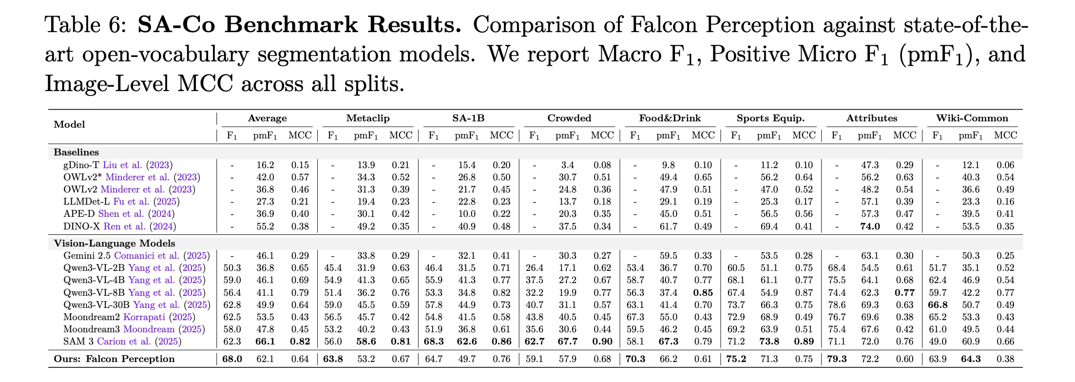
PBench: Profiling Capabilities Past Saturated Baselines
To measure progress, TII analysis crew launched PBench, a benchmark that organizes samples into 5 ranges of semantic complexity to disentangle mannequin failure modes.
Foremost Outcomes: Falcon Notion vs. SAM 3 (Macro-F1)
Benchmark Cut up
SAM 3
Falcon Notion (600M)
L0: Easy Objects
64.3
65.1
L1: Attributes
54.4
63.6
L2: OCR-Guided
24.6
38.0
L3: Spatial Understanding
31.6
53.5
L4: Relations
33.3
49.1
Dense Cut up
58.4
72.6
Falcon Notion considerably outperforms SAM 3 on advanced semantic duties, notably exhibiting a +21.9 level achieve on spatial understanding (Stage 3).
https://arxiv.org/pdf/2603.27365
FalconOCR: The 300M Doc specialist
TII crew additionally prolonged this early-fusion recipe to FalconOCR, a compact 300M-parameter mannequin initialized from scratch to prioritize fine-grained glyph recognition. FalconOCR is aggressive with a number of bigger proprietary and modular OCR programs:
olmOCR: Achieves 80.3% accuracy, matching or exceeding Gemini 3 Professional (80.2%) and GPT 5.2 (69.8%).
OmniDocBench: Reaches an total rating of 88.64, forward of GPT 5.2 (86.56) and Mistral OCR 3 (85.20), although it trails the highest modular pipeline PaddleOCR VL 1.5 (94.37).
Key Takeaways
Unified Early-Fusion Structure: Falcon Notion replaces modular encoder-decoder pipelines with a single dense Transformer that processes picture patches and textual content tokens in a shared parameter area from the primary layer. It makes use of a hybrid consideration masks—bidirectional for visible tokens and causal for activity tokens—to behave concurrently as a imaginative and prescient encoder and an autoregressive decoder.
Chain-of-Notion Sequence: The mannequin serializes occasion segmentation right into a structured sequence , which forces it to resolve spatial place and measurement as a conditioning sign earlier than producing the pixel-level masks.
Specialised Heads and GGROPE: To handle dense spatial information, the mannequin makes use of Fourier Characteristic encoders for high-dimensional coordinate mapping and Golden Gate ROPE (GGROPE) to allow isotropic 2D spatial consideration. The Muon optimizer is employed for these specialised heads to steadiness studying charges in opposition to the pre-trained spine.
Semantic Efficiency Positive aspects: On the brand new PBench benchmark, which disentangles semantic capabilities (Ranges 0-4), the 600M mannequin demonstrates vital positive factors over SAM 3 in advanced classes, together with a +13.4 level lead in OCR-guided queries and a +21.9 level lead in spatial understanding.
Excessive-Effectivity OCR Extension: The structure scales all the way down to Falcon OCR, a 300M-parameter mannequin that achieves 80.3% on olmOCR and 88.64 on OmniDocBench. It matches or exceeds the accuracy of a lot bigger programs like Gemini 3 Professional and GPT 5.2 whereas sustaining excessive throughput for large-scale doc processing.
Samsung Climate v1.7.30.8 updates a number of UI parts, together with new particular icons for the pollen card.
The moon section card is now extra compact, whereas wind and stress playing cards function redesigned graphics.
New fast toggles on the radar map now hyperlink on to particular views on The Climate Channel’s web site.
Samsung Galaxy smartphones, equivalent to the newest Galaxy S26 collection, include the Samsung Climate app preloaded. It’s a kind of uncommon apps from the corporate that look nice and get the job achieved. Samsung has up to date the Climate app to v1.7.30.8, bringing some good UI adjustments, equivalent to newer icons for varied playing cards and fast toggles for the Radar map.
Beginning off, the Pollen card on Samsung Climate has been up to date with new icons. Out goes the generic translucent leaf icon, and we now have particular opaque icons for Tree, Grass, and Ragweed that make it simpler to get info at a look — although Samsung may do a greater job at depicting the depth with the icons.
The Wind and Stress playing cards additionally see new graphics, although opinion could possibly be divided on whether or not these new icons are as useful. The older icons had been simpler to look at, with outstanding textual content that’s simple to learn.
Don’t wish to miss the very best from Android Authority?
The Moon and Radar playing cards additionally see adjustments. The Moon card takes much less area now, because the moonset and moonrise instances at the moment are positioned facet by facet for much less wasted area.
The Radar card reveals extra icons on the backside of the map for interplay. We now have icons for the 6-hour forecast, radar, cloud, and temperature. Every of those icons opens the precise sort of radar map on The Climate Channel‘s web site.
All of those adjustments are dwell within the app, so replace your Climate app from the Galaxy Retailer immediately.
Thanks for being a part of our group. Learn our Remark Coverage earlier than posting.
A uncommon “sungrazer” comet is about to move very near our star and will change into seen in daylight — or it may utterly disintegrate earlier than our eyes. Both manner, there could possibly be one thing particular to see within the night time sky, with a big tail probably seen late this week.
C/2026 A1 (MAPS) belongs to a particular household of comets referred to as Kreutz “sungrazers,” so referred to as as a result of they get very near the solar, lighting up brightly however usually breaking into smaller items. There are round 3,500 members of the Kreutz household, all of that are regarded as fragments of a single big comet that obtained too near the solar about 1,700 years in the past, in line with Dwell Science’s sister web site House.com.
C/2026 A1 (MAPS) is anticipated to get inside 98,000 miles (158,000 km) of the solar’s floor and move by the decrease areas of the solar’s outer ambiance, or corona, at 9:30 a.m. EDT (13:30 UTC) Saturday (April 4), in line with the British Astronomical Affiliation (BAA). In response to the European House Company, many Kreutz sungrazers evaporate, but when they survive, they might placed on a spectacular present.
As a result of C/2026 A1 (MAPS) is touring into the solar’s glare, it will likely be tough to see earlier than April 4. If it survives its shut encounter with the solar — even when it fragments — it may change into seen for a short while after sundown within the evenings that comply with. Except it breaks aside earlier than it will get near the solar, there will probably be a chance of seeing a probably massive and vibrant tail within the western night sky beginning round April 9, in line with the BAA.
If that happens, Comet C/2026 A1 (MAPS) would be the first of two comets seen in April, with the possible dimmer however extra predictable C/2025 R3 (PanSTARRS) set to change into a simple binocular goal near April 20.
Get the world’s most fascinating discoveries delivered straight to your inbox.
assume that linear regression is about becoming a line to knowledge.
However mathematically, that’s not what it’s doing.
It’s discovering the closest attainable vector to your goal inside the area spanned by options.
To know this, we have to change how we have a look at our knowledge.
In Half 1, we’ve received a fundamental thought of what a vector is and explored the ideas of dot merchandise and projections.
Now, let’s apply these ideas to unravel a linear regression downside.
We now have this knowledge.
Picture by Creator
The Common Manner: Function Area
Once we attempt to perceive linear regression, we typically begin with a scatter plot drawn between the unbiased and dependent variables.
Every level on this plot represents a single row of knowledge. We then attempt to match a line via these factors, with the aim of minimizing the sum of squared residuals.
To resolve this mathematically, we write down the price operate equation and apply differentiation to search out the precise formulation for the slope and intercept.
As we already mentioned in my earlier a number of linear regression (MLR) weblog, that is the usual option to perceive the issue.
That is what we name as a characteristic area.
Picture by Creator
After doing all that course of, we get a worth for the slope and intercept. Right here we have to observe one factor.
Allow us to say ŷᵢ is the anticipated worth at a sure level. We now have the slope and intercept worth, and now in response to our knowledge, we have to predict the value.
If ŷᵢ is the anticipated worth for Home 1, we calculate it through the use of
[ beta_0 + beta_1 cdot text{size} ]
What have we accomplished right here? We now have a measurement worth, and we’re scaling it with a sure quantity, which we name the slope (β₁), to get the worth as close to to the unique worth as attainable.
We additionally add an intercept (β₀) as a base worth.
Now let’s keep in mind this level, and we’ll transfer to the subsequent perspective.
A Shift in Perspective
Let’s have a look at our knowledge.
Now, as an alternative of contemplating Value and Measurement as axes, let’s take into account every home as an axis.
We now have three homes, which suggests we are able to deal with Home A because the X-axis, Home B because the Y-axis, and Home C because the Z-axis.
Then, we merely plot our factors.
Picture by Creator
Once we take into account the dimensions and worth columns as axes, we get three factors, the place every level represents the dimensions and worth of a single home.
Nonetheless, after we take into account every home as an axis, we get two factors in a third-dimensional area.
One level represents the sizes of all three homes, and the opposite level represents the costs of all three homes.
That is what we name the column area, and that is the place the linear regression occurs.
From Factors to Instructions
Now let’s join our two factors to the origin and now we name them as vectors.
Picture by Creator
Okay, let’s decelerate and have a look at what we have now accomplished and why we did it.
As a substitute of a traditional scatter plot the place measurement and worth are the axes (Function Area), we thought of every home as an axis and plotted the factors (Column Area).
We at the moment are saying that linear regression occurs on this Column Area.
You is perhaps considering: Wait, we study and perceive linear regression utilizing the normal scatter plot, the place we reduce the residuals to discover a best-fit line.
Sure, that’s appropriate! However in Function Area, linear regression is solved utilizing calculus. We get the formulation for the slope and intercept utilizing partial differentiation.
For those who keep in mind my earlier weblog on MLR, we derived the formulation for the slopes and intercepts after we had two options and a goal variable.
You may observe how messy it was to calculate these formulation utilizing calculus. Now think about in case you have 50 or 100 options; it turns into complicated.
By switching to Column Area, we alter the lens via which we view regression.
We have a look at our knowledge as vectors and use the idea of projections. The geometry stays precisely the identical whether or not we have now 2 options or 2,000 options.
So, if calculus will get that messy, what’s the actual good thing about this unchanging geometry? Let’s talk about precisely what occurs in Column Area.”
Why This Perspective Issues
Now that we have now an thought of what Function Area and Column Area are, let’s deal with the plot.
We now have two factors, the place one represents the sizes and the opposite represents the costs of the homes.
Why did we join them to the origin and take into account them vectors?
As a result of, as we already mentioned, in linear regression we’re discovering a quantity (which we name the slope or weight) to scale our unbiased variable.
We need to scale the Measurement so it will get as near the Value as attainable, minimizing the residual.
You can’t visually scale a floating level; you’ll be able to solely scale one thing when it has a size and a path.
By connecting the factors to the origin, they develop into vectors. Now they’ve each magnitude and path, and we already know that we are able to scale vectors.
Picture by Creator
Okay, we established that we deal with these columns as vectors as a result of we are able to scale them, however there’s something much more vital to study right here.
Let’s have a look at our two vectors: the Measurement vector and the Value vector.
First, if we have a look at the Measurement vector (1, 2, 3), it factors in a really particular path based mostly on the sample of its numbers.
From this vector, we are able to perceive that Home 2 is twice as massive as Home 1, and Home 3 is thrice as massive.
There’s a particular 1:2:3 ratio, which forces the Measurement vector to level in a single actual path.
Now, if we have a look at the Value vector, we are able to see that it factors in a barely completely different path than the Measurement vector, based mostly by itself numbers.
The path of an arrow merely exhibits us the pure, underlying sample of a characteristic throughout all our homes.
If our costs have been precisely (2, 4, 6), then our Value vector would lie precisely in the identical path as our Measurement vector. That might imply measurement is an ideal, direct predictor of worth.
Picture by Creator
However in actual life, that is hardly ever attainable. The worth of a home isn’t just depending on measurement; there are numerous different components that have an effect on it, which is why the Value vector factors barely away.
That angle between the 2 vectors (1,2,3) and (4,8,9) represents the real-world noise.
The Geometry Behind Regression
Picture by Creator
Now, we use the idea of projections that we realized in Half 1.
Let’s take into account our Value vector (4, 8, 9) as a vacation spot we need to attain. Nonetheless, we solely have one path we are able to journey which is the trail of our Measurement vector (1, 2, 3).
If we journey alongside the path of the Measurement vector, we are able to’t completely attain our vacation spot as a result of it factors in a distinct path.
However we are able to journey to a particular level on our path that will get us as near the vacation spot as attainable.
The shortest path from our vacation spot dropping all the way down to that actual level makes an ideal 90-degree angle.
In Half 1, we mentioned this idea utilizing the ‘freeway and residential’ analogy.
We’re making use of the very same idea right here. The one distinction is that in Half 1, we have been in a 2D area, and right here we’re in a 3D area.
I referred to the characteristic as a ‘manner’ or a ‘freeway’ as a result of we solely have one path to journey.
This distinction between a ‘manner’ and a ‘path’ will develop into a lot clearer later after we add a number of instructions!
A Easy Technique to See This
We are able to already observe that that is the very same idea as vector projections.
We derived a components for this in Half 1. So, why wait?
Let’s simply apply the components, proper?
No. Not but.
There’s something essential we have to perceive first.
In Half 1, we have been coping with a 2D area, so we used the freeway and residential analogy. However right here, we’re in a 3D area.
To know it higher, let’s use a brand new analogy.
Think about this 3D area as a bodily room. There’s a lightbulb hovering within the room on the coordinates (4, 8, 9).
The trail from the origin to that bulb is our Value vector which we name as a goal vector.
We need to attain that bulb, however our actions are restricted.
We are able to solely stroll alongside the path of our Measurement vector (1, 2, 3), shifting both ahead or backward.
Based mostly on what we realized in Half 1, you may say, ‘Let’s simply apply the projection components to search out the closest level on our path to the bulb.’
And you’ll be proper. That’s the absolute closest we are able to get to the bulb in that path.
Why We Want a Base Worth?
However earlier than we transfer ahead, we must always observe yet another factor right here.
We already mentioned that we’re discovering a single quantity (a slope) to scale our Measurement vector so we are able to get as near the Value vector as attainable. We are able to perceive this with a easy equation:
Value = β₁ × Measurement
However what if the dimensions is zero? Regardless of the worth of β₁ is, we get a predicted worth of zero.
However is that this proper? We’re saying that if the dimensions of a home is 0 sq. toes, the value of the home is 0 {dollars}.
This isn’t appropriate as a result of there needs to be a base worth for every home. Why?
As a result of even when there is no such thing as a bodily constructing, there’s nonetheless a worth for the empty plot of land it sits on. The worth of the ultimate home is closely depending on this base plot worth.
We name this base worth β0. In conventional algebra, we already know this because the intercept, which is the time period that shifts a line up and down.
So, how can we add a base worth in our 3D room? We do it by including a Base Vector.
Combining Instructions
GIF by Creator
Now we have now added a base vector (1, 1, 1), however what is definitely accomplished utilizing this base vector?
From the above plot, we are able to observe that by including a base vector, we have now yet another path to maneuver in that area.
We are able to transfer in each the instructions of the Measurement vector and the Base vector.
Don’t get confused by them as “methods”; they’re instructions, and it is going to be clear as soon as we get to a degree by shifting in each of them.
With out the bottom vector, our base worth was zero. We began with a base worth of zero for each home. Now that we have now a base vector, let’s first transfer alongside it.
For instance, let’s transfer 3 steps within the path of the Base vector. By doing so, we attain the purpose (3, 3, 3). We’re presently at (3, 3, 3), and we need to attain as shut as attainable to our Value vector.
This implies the bottom worth of each home is 3 {dollars}, and our new start line is (3, 3, 3).
Subsequent, let’s transfer 2 steps within the path of our Measurement vector (1, 2, 3). This implies calculating 2 * (1, 2, 3) = (2, 4, 6).
Subsequently, from (3, 3, 3), we transfer 2 steps alongside the Home A axis, 4 models alongside the Home B axis, and 6 steps alongside the Home C axis.
Principally, we’re including the vectors right here, and the order doesn’t matter.
Whether or not we transfer first via the bottom vector or the dimensions vector, it will get us to the very same level. We simply moved alongside the bottom vector first to grasp the thought higher!
The Area of All Doable Predictions
This fashion, we use each the instructions to get as near our Value vector. Within the earlier instance, we scaled the Base vector by 3, which suggests right here β0 = 3, and we scaled the Measurement vector by 2, which suggests β1 = 2.
From this, we are able to observe that we’d like the perfect mixture of β0 and β1 in order that we are able to know what number of steps we journey alongside the bottom vector and what number of steps we journey alongside the dimensions vector to succeed in that time which is closest to our Value vector.
On this manner, if we attempt all of the completely different mixtures of β0 and β₁, then we get an infinite variety of factors, and let’s see what it appears like.
GIF by Creator
We are able to see that each one the factors fashioned by the completely different mixtures of β0 and β1 alongside the instructions of the Base vector and Measurement vector kind a flat 2D airplane in our 3D area.
Now, we have now to search out the purpose on that airplane which is nearest to our Value vector.
We already know how you can get to that time. As we mentioned in Half 1, we discover the shortest path through the use of the idea of geometric projections.
Now we have to discover the precise level on the airplane which is nearest to the Value vector.
We already mentioned this in Half 1 utilizing our ‘dwelling and freeway’ analogy, the place the shortest path from the freeway to the house fashioned a 90-degree angle with the freeway.
There, we moved in a single dimension, however right here we’re shifting on a 2D airplane. Nonetheless, the rule stays the identical.
The shortest distance between the tip of our worth vector and a degree on the airplane is the place the trail between them kinds an ideal 90-degree angle with the airplane.
GIF by Creator
From a Level to a Vector
Earlier than we dive into the maths, allow us to make clear precisely what is going on in order that it feels straightforward to comply with.
Till now, we have now been speaking about discovering the precise level on our airplane that’s closest to the tip of our goal worth vector. However what can we truly imply by this?
To succeed in that time, we have now to journey throughout our airplane.
We do that by shifting alongside our two accessible instructions, that are our Base and Measurement vectors, and scaling them.
Whenever you scale and add two vectors collectively, the result’s at all times a vector!
If we draw a straight line from the middle on the origin on to that actual level on the airplane, we create what known as the Prediction Vector.
Transferring alongside this single Prediction Vector will get us to the very same vacation spot as taking these scaled steps alongside the Base and Measurement instructions.
The Vector Subtraction
Now we have now two vectors.
We need to know the precise distinction between them. In linear algebra, we discover this distinction utilizing vector subtraction.
Once we subtract our Prediction from our Goal, the result’s our Residual Vector, often known as the Error Vector.
For this reason that dotted pink line isn’t just a measurement of distance. It’s a vector itself!
Once we deal in characteristic area, we attempt to reduce the sum of squared residuals. Right here, by discovering the purpose on the airplane closest to the value vector, we’re not directly in search of the place the bodily size of the residual path is the bottom!
Linear Regression Is a Projection
Now let’s begin the maths.
[ text{Let’s start by representing everything in matrix form.} ]
[
X =
begin{bmatrix}
1 & 1
1 & 2
1 & 3
end{bmatrix}
quad
y =
begin{bmatrix}
4
8
9
end{bmatrix}
quad
beta =
begin{bmatrix}
b_0
b_1
end{bmatrix}
]
[
text{Here, the columns of } X text{ represent the base and size directions.}
]
[
text{And we are trying to combine them to reach } y.
]
[
hat{y} = Xbeta
]
[
= b_0
begin{bmatrix}
1
1
1
end{bmatrix}
+
b_1
begin{bmatrix}
1
2
3
end{bmatrix}
]
[
text{Every prediction is just a combination of these two directions.}
]
[
e = y – Xbeta
]
[
text{This error vector is the gap between where we want to be.}
]
[
text{And where we actually reach.}
]
[
text{For this gap to be the shortest possible,}
]
[
text{it must be perfectly perpendicular to the plane.}
]
[
text{This plane is formed by the columns of } X.
]
[
X^T e = 0
]
[
text{Now we substitute ‘e’ into this condition.}
]
[
X^T (y – Xbeta) = 0
]
[
X^T y – X^T X beta = 0
]
[
X^T X beta = X^T y
]
[
text{By simplifying we get the equation.}
]
[
beta = (X^T X)^{-1} X^T y
]
[
text{Now we compute each part step by step.}
]
[
X^T =
begin{bmatrix}
1 & 1 & 1
1 & 2 & 3
end{bmatrix}
]
[
X^T X =
begin{bmatrix}
3 & 6
6 & 14
end{bmatrix}
]
[
X^T y =
begin{bmatrix}
21
47
end{bmatrix}
]
[
text{computing the inverse of } X^T X.
]
[
(X^T X)^{-1}
=
frac{1}{(3 times 14 – 6 times 6)}
begin{bmatrix}
14 & -6
-6 & 3
end{bmatrix}
]
[
=
frac{1}{42 – 36}
begin{bmatrix}
14 & -6
-6 & 3
end{bmatrix}
]
[
=
frac{1}{6}
begin{bmatrix}
14 & -6
-6 & 3
end{bmatrix}
]
[
text{Now multiply this with } X^T y.
]
[
beta =
frac{1}{6}
begin{bmatrix}
14 & -6
-6 & 3
end{bmatrix}
begin{bmatrix}
21
47
end{bmatrix}
]
[
=
frac{1}{6}
begin{bmatrix}
14 cdot 21 – 6 cdot 47
-6 cdot 21 + 3 cdot 47
end{bmatrix}
]
[
=
frac{1}{6}
begin{bmatrix}
294 – 282
-126 + 141
end{bmatrix}
=
frac{1}{6}
begin{bmatrix}
12
15
end{bmatrix}
]
[
=
begin{bmatrix}
2
2.5
end{bmatrix}
]
[
text{With these values, we can finally compute the exact point on the plane.}
]
[
hat{y} =
2
begin{bmatrix}
1
1
1
end{bmatrix}
+
2.5
begin{bmatrix}
1
2
3
end{bmatrix}
=
begin{bmatrix}
4.5
7.0
9.5
end{bmatrix}
]
[
text{And this point is the closest possible point on the plane to our target.}
]
We received the purpose (4.5, 7.0, 9.5). That is our prediction.
This level is the closest to the tip of the value vector, and to succeed in that time, we have to transfer 2 steps alongside the bottom vector, which is our intercept, and a couple of.5 steps alongside the dimensions vector, which is our slope.
What Modified Was the Perspective
Let’s recap what we have now accomplished on this weblog. We haven’t adopted the common technique to unravel the linear regression downside, which is the calculus technique the place we attempt to differentiate the equation of the loss operate to get the equations for the slope and intercept.
As a substitute, we selected one other technique to unravel the linear regression downside which is the tactic of vectors and projections.
We began with a Value vector, and we would have liked to construct a mannequin that predicts the value of a home based mostly on its measurement.
By way of vectors, that meant we initially solely had one path to maneuver in to foretell the value of the home.
Then, we additionally added the Base vector by realizing there needs to be a baseline beginning worth.
Now we had two instructions, and the query was how shut can we get to the tip of the Value vector by shifting in these two instructions?
We aren’t simply becoming a line; we’re working inside an area.
In characteristic area: we reduce error
In column area: we drop perpendiculars
By utilizing completely different mixtures of the slope and intercept, we received an infinite variety of factors that created a airplane.
The closest level, which we would have liked to search out, lies someplace on that airplane, and we discovered it through the use of the idea of projections and the dot product.
By means of that geometry, we discovered the proper level and derived the Regular Equation!
Chances are you’ll ask, “Don’t we get this regular equation through the use of calculus as nicely?” You might be precisely proper! That’s the calculus view, however right here we’re coping with the geometric linear algebra view to actually perceive the geometry behind the maths.
Linear regression isn’t just optimization.
It’s projection.
I hope you realized one thing from this weblog!
For those who assume one thing is lacking or could possibly be improved, be happy to depart a remark.
For those who haven’t learn Half 1 but, you’ll be able to learn it right here. It covers the fundamental geometric instinct behind vectors and projections.
REDLANDS, CALIF. — For the town of Cleveland’s chief innovation and know-how officer (CITO), Elizabeth Crowe, creating an open knowledge administration platform in a digitally challenged atmosphere was like being in an episode of the TV present “Hoarders.” The town’s departments had knowledge residing in every single place, from native machines to clusters of sticky notes. Because the lead on Cleveland’s open knowledge initiative, Crowe dug into the present IT infrastructure for the town and uncovered a staggering 130 enterprise techniques.
Tasked by Main Justin Bibb, Crowe has taken on the monumental duties of bringing the town’s public places of work into the twenty first century, constructing knowledge dashboards and deploying an open knowledge coverage for the town. Previous to her appointment as interim CITO in February, Crowe was named director and founding father of the Workplace of City Analytics and Innovation (City AI) in August 2022.
“I joked with the mayor that he put me on a path the place I did not should construct the home,” Crowe stated. “I needed to go mill the lumber to then construct the home, to then work out how we’ll deploy some dashboards within the metropolis.”
To set the stage for the challenges Crowe confronted getting metropolis corridor updated with know-how, she defined that Cleveland’s earlier mayor did not even have an digital calendar. “We didn’t get public-facing emails for the town till 2014, and our police division didn’t get it till 2018. We now have been a bit little bit of Luddites,” Crowe defined throughout final week’s Public Sector CIO Summit, held by geographic info system (GIS) software program firm Esri.
Gaining mayoral help for open knowledge
To modernize the native authorities places of work, Crowe stated her group members assessed the enterprise issues and recognized their No. 1 directive — attending to open knowledge. Bibb’s second government order established an open knowledge coverage and open knowledge governance board, a transfer that offered Crowe with the official backing to inform governmental departments they would wish to get on board with the info administration initiative.
“This government order declared knowledge as a strategic asset that’s essential to assembly the calls for of a contemporary authorities,” Crowe stated.
Thus, the Metropolis of Cleveland Open Knowledge Coverage was born in December 2023. In response to the coverage, “By leveraging knowledge as a strategic asset, the Metropolis can tackle challenges proactively, optimize useful resource allocation, enhance service supply, and enhance transparency.” As well as, all metropolis of Cleveland departments have been tasked with adopting a framework that features a knowledge stock, knowledge requirements, knowledge use and infrastructure, open knowledge and a governance board.
With the mayor’s government order in place, the subsequent step for Crowe was to create a list of what knowledge was already accessible inside Cleveland’s native authorities.
“Generally I’d go to individuals and say, ‘The place is your knowledge?’ And they might level, actually, to the server beneath their desk. I needed to begin telling them, ‘In the event you kick your knowledge while you get your espresso within the morning, we’re doing it flawed. Let’s give you a greater approach to sort out this knowledge right here.'”
Crowe stated she found knowledge was residing in disparate areas, from Excel spreadsheets to sticky notes surrounding one workers member’s monitor.
Establishing the tech stack
After inventorying Cleveland’s public knowledge, Crowe’s group got down to choose distributors and enterprise knowledge dashboard software program. “We had knowledge on-prem, we had knowledge within the cloud, however we had no analytics warehouse that we might then use,” she defined.
When it got here to discovering a vendor, Crowe stated her group targeted on the overarching purpose of “attending to open knowledge” whereas “contemplating every layer of our tech stack and treating every section of the info individually.”
As a Microsoft store, Crowe’s group selected Microsoft Azure Industrial Cloud, together with Microsoft Energy BI, an information visualization and enterprise intelligence software. The group additionally chosen Esri as its GIS mapping software program vendor.
“I had a greenfield [environment],” Crowe stated. “The cool half a few greenfield is I can construct a contemporary tech stack that has ready us for the subsequent wave of analytics work. The problem of a greenfield is you do not have something to begin with. So, you do not have a framework, and you do not have a governance.”
Upskilling throughout Cleveland
As soon as vendor choice was established, Crowe assessed the technical abilities of her 16 group members to find out the place they may “develop into specialists” and prepare different departments, and the place she wanted to fill in gaps by figuring out “a bench of analysts across the metropolis.”
“We knew that we wanted of us who would speak about knowledge, who might educate about knowledge, who knew and understood how you can use instruments in a contemporary tech stack,” Crowe stated. Her group tasked the greater than 30 departments throughout the town with figuring out “knowledge leads” — staff with levels in areas equivalent to knowledge analytics who might meet with Crowe’s group month-to-month for coaching {and professional} growth.
Lastly, Crowe’s group established an information coverage based mostly on a stage system from one via 4. Stage one is knowledge that is open to the general public; stage two is operational info like what number of assist desk tickets are available; stage three pertains to compliance knowledge equivalent to HIPAA and Household Academic Rights and Privateness Act (FERPA); and stage 4 is restricted and confidential knowledge.
This month marks the two-year anniversary of Cleveland’s open knowledge portal, which Crowe’s group launched in April 2024. Among the many public-facing dashboards is a Cleveland Cemetery Viewer software, which lets residents find burial plots, and a web-based 311 dashboard to lookup service requests. The group can be engaged on a property insights software that can combine knowledge from 15 metropolis techniques into an internet map — customers will be capable of seek for details about property possession, transfers and gross sales. However that is simply the tip of the iceberg, Crowe stated.
“These are my high three, however we have a ton of different public instruments that we have been in a position to construct and develop and launch.”
Early within the first Trump administration, the authorized journalist Benjamin Wittes coined probably the greatest descriptions of how President Donald Trump governs: “malevolence tempered by incompetence.” Trump, as Wittes initially wrote, typically issued government orders that weren’t vetted by legal professionals or coverage consultants — and thus had been susceptible to lawsuits and infrequently achieved little or no. And this penchant for taking seemingly daring actions that collapse as soon as they’re uncovered to the true world pervades each of Trump’s administrations.
Nobody embodied Trump’s model of incompetent malice greater than outgoing Legal professional Common Pam Bondi, who, as Trump introduced Thursday, “can be transitioning” to a “new job within the personal sector.” In her 15 months because the nation’s high authorized official, Bondi flouted norms, stretching again to the top of the Nixon administration, which sought to insulate federal prosecutors from political management by the White Home. However her precise makes an attempt to make use of the Division of Justice to hunt revenge towards Trump’s perceived enemies incessantly floundered on the shores of dangerous lawyering.
Bondi could also be greatest recognized for saying, in a February 2025 interview with Fox Information, {that a} listing of intercourse offender Jeffrey Epstein’s purchasers was “sitting on my desk proper now” — months earlier than the DOJ later claimed that this listing doesn’t exist. After she was requested about her mishandling of the Epstein recordsdata in a congressional listening to, she informed lawmakers that they shouldn’t even be speaking about Epstein as a result of “the Dow is over 50,000 proper now.” (As of this writing, the Dow Jones Industrial Common sits at 46,371.57.)
Take into account, as effectively, the Trump DOJ’s makes an attempt to prosecute former FBI Director James Comey and New York Legal professional Common Letitia James, two officers who Trump loathes as a result of they investigated allegedly criminal activity by the president. Each prosecutions had been dismissed by a federal courtroom, nevertheless, after a choose decided that Lindsey Halligan, the previous insurance coverage lawyer that this administration tried to put in as a high federal prosecutor in Virginia, was by no means lawfully appointed.
Equally, when the Trump administration ordered 1000’s of federal regulation enforcement officers to occupy town of Minneapolis and to arrest many immigrants in that metropolis, a reliable legal professional basic would have acknowledged that these mass arrests would set off an array of authorized proceedings, and would have preemptively detailed extra legal professionals to Minnesota to deal with the elevated caseload. As a substitute, the US Legal professional’s Workplace in Minnesota was virtually comically understaffed, and utterly unprepared for an array of courtroom orders, requiring the administration to launch lots of the immigrants it had simply arrested.
Federal judges criticized the Justice Division’s incompetence of their opinions — the chief choose of the native federal district courtroom wrote that the Trump administration “determined to ship 1000’s of brokers to Minnesota to detain aliens with out making any provision for coping with the tons of of habeas petitions and different lawsuits that had been positive to outcome.” One DOJ lawyer, who was assigned an inconceivable workload of 88 instances in a single month, informed a choose that she generally wished she’d be held in contempt of courtroom in order that she may sleep in jail.
At instances, the ineptitude of Bondi’s Justice Division even endangered the Republican Occasion’s capability to carry onto political energy. Final November, a federal courtroom in Texas struck down a Republican gerrymander that’s anticipated to realize the GOP 5 extra US Home seats after the 2026 midterms. The courtroom’s opinion, authored by a Trump-appointed choose, relied on a letter from one in every of Bondi’s high lieutenants, which successfully ordered the state of Texas to redraw its maps for racial causes which might be forbidden by the Structure.
Although the Supreme Court docket ultimately reinstated the gerrymander, the decrease courtroom’s determination was well-rooted in Supreme Court docket precedents questioning racially motivated legal guidelines. All of this drama would have been prevented if Bondi’s DOJ had by no means despatched its letter, which the choose mentioned was “difficult to unpack” as a result of “it comprises so many factual, authorized, and typographical errors,” Texas’s Republican gerrymander would have by no means been in any hazard.
This listing is only the start. Not each Republican legal professional basic loyal to Trump would have made such primary errors in finishing up his agenda. And there’s no assure that Bondi’s successor will share her ineptitude. So Trump’s opponents could wish to wait and see what comes subsequent earlier than they have fun Bondi’s humiliation.
Bondi’s ouster offers Trump an opportunity to put a reliable loyalist accountable for DOJ
Bondi’s bumbling administration of the Justice Division would have mattered extra if Republicans didn’t have a agency grip on the federal judiciary. For the second, not less than, lawsuits difficult many unlawful detentions in Minnesota are on maintain due to a determination by two Republican appellate judges holding that these detentions are, in reality, legally mandated. The Texas courtroom’s determination towards that state’s gerrymander was blocked by a Republican Supreme Court docket.
Nonetheless, Bondi’s incompetence is more likely to plague the DOJ for a very long time, despite the fact that she not leads it. Federal judges have traditionally handled Justice Division legal professionals with a level of deference, as a result of for many years the DOJ held a well-deserved repute for being candid with judges and for hiring extremely expert legal professionals. However now many judges are brazenly questioning the Justice Division of their opinions. That implies that rank-and-file Justice Division legal professionals must spend numerous hours shoring up claims that federal judges would have merely believed previously.
In the meantime, the worst-case state of affairs for Trump’s political enemies, and for anybody else who the Justice Division decides to focus on for political causes, is that Bondi might be changed by a succesful advocate. (The total listing of attainable candidates to exchange Bondi just isn’t but recognized, however some early information studies point out that EPA administrator Lee Zeldin is into account).
A reliable legal professional basic would have made positive {that a} lawfully appointed prosecutor introduced costs towards Comey and James. A reliable legal professional basic may need selectively leaked Epstein paperwork that point out Democrats, moderately than inspiring an act of Congress requiring the entire paperwork to be launched. And a reliable legal professional basic would deal with DOJ legal professionals’ time as valuable, as a result of each minute a prosecutor spends on pointless work is time they’ll’t spend advancing Trump’s agenda.
It stays to be seen who Trump will choose to exchange the maladroit Bondi. However there’s hardly a scarcity of extremely partisan Republican legal professionals who’re really good at their jobs. Trump may discover somebody like his first-term Legal professional Common Invoice Barr, who was a very succesful advocate for MAGA’s agenda. And, if that occurs, anybody unlucky to wind up on Trump’s enemies listing will miss Pam Bondi.
The mission’s Orion capsule aced a vital translunar injection (TLI) burn this night (April 2), firing its essential engine to go away Earth orbit and head towards our planet’s pure satellite tv for pc.
It was an enormous milestone for the Artemis 2 mission, and one in all its crewmembers marked it with some poignant phrases.
The view from NASA’s Artemis 2 Orion capsule through the mission’s essential translunar injection burn on April 2, 2026. (Picture credit score: NASA)
“With that profitable TLI, the crew is feeling fairly good up right here on our approach to the moon, and we simply wished to speak to everybody across the planet who’s labored to make Artemis potential that we firmly felt the ability of your perseverance throughout each second of that burn,” Artemis 2 astronaut Jeremy Hansen, of the Canadian House Company, mentioned simply after the maneuver.
“Humanity has as soon as once more proven what we’re able to, and it is your hopes for the longer term that carry us now on this journey across the moon,” he added.
Artemis 2 launched Wednesday night (April 1) from NASA’s Kennedy House Middle in Florida, sending 4 astronauts aloft on the first-ever crewed flight of Orion and its House Launch System (SLS) rocket. The duo had flown collectively simply as soon as earlier than, on the uncrewed Artemis 1 mission to lunar orbit in 2022.
Orion and its occupants — Hansen and NASA’s Reid Wiseman, Victor Glover and Christina Koch — stayed in Earth orbit for greater than 24 hours, testing the capsule’s numerous methods forward of its deliberate plunge into deep area.
Breaking area information, the most recent updates on rocket launches, skywatching occasions and extra!
This afternoon, Artemis 2’s mission administration group declared the spacecraft match for this big leap, greenlighting the TLI burn. So, beginning at 7:49 p.m. EDT (2349 GMT), Orion fired its essential engine for 5 minutes and 50 seconds, placing it on a trajectory to loop across the moon after which head again to Earth — with out the necessity for another main maneuvers.
“Our TLI burn, the burn that will get us going to the moon, can be our deorbit burn,” Koch mentioned in a NASA interview earlier than launch. “As quickly as we take that burn, now we have purchased off on principally the remainder of the mission.”
The TLI burn used Orion’s essential orbital maneuvering engine, which was salvaged from NASA’s area shuttle program and upgraded for an Artemis journey to the moon. The engine has flown in area 19 instances earlier than on three totally different area shuttles. In the event you strapped it to a automotive, it will speed up you from zero to 60 mph (97 kph) in 2.7 seconds.
(Orion has three major strategies of propulsion: its essential engine and a set of eight smaller auxiliary engines, that are on its European Service Module, and a set of response management thrusters on the capsule itself.)
The foremost milestones of the Artemis 2 moon mission. (Picture credit score: NASA)
Artemis 2 is now on monitor to turn into the primary crewed mission to go to the moon since Apollo 17, which landed on the lunar floor in December 1972. Koch is the primary girl ever to go away low Earth orbit, and Glover and Hansen are the primary particular person of shade and the primary non-American, respectively, to take action. (The Apollo astronauts had been all white males.)
Orion will loop across the moon on Day 6 of the mission — about 5 days, one hour and half-hour after liftoff. The Artemis 2 quartet will set one other report within the course of, getting farther away from Earth than any people ever have earlier than. They’re going to beat the mark set by the Apollo 13 astronauts, who traveled a most of 248,655 miles (400,171 kilometers) from our planet after struggling an in-flight anomaly that derailed their moon-landing plans.
Artemis 2 will come dwelling on Day 10 of the mission, splashing down within the Pacific Ocean off the coast of San Diego. Full success on this check mission will assist pave the best way towards the Artemis program‘s first crewed moon touchdown, on Artemis 4 in 2028, and the development of a lunar base a number of years after that, if all goes in line with plan.
I wish to begin a collection on utilizing Stata’s random-number operate. Stata the truth is has ten random-number features:
runiform() generates rectangularly (uniformly) distributed random quantity over [0,1).
rbeta(a,b) generates beta-distribution beta(a, b) random numbers.
rbinomial(n,p) generates binomial(n, p) random numbers, where n is the number of trials and p the probability of a success.
rchi2(df) generates χ2 with df degrees of freedom random numbers.
rgamma(a,b) generates Γ(a, b) random numbers, where a is the shape parameter and b, the scale parameter.
rhypergeometric(N,K,n) generates hypergeometric random numbers, where N is the population size, K is the number of in the population having the attribute of interest, and n is the sample size.
rnbinomial(n,p) generates negative binomial — the number of failures before the nth success — random numbers, where p is the probability of a success. (n can also be noninteger.)
rnormal(μ,σ) generates Gaussian normal random numbers.
rpoisson(m) generates Poisson(m) random numbers.
rt(df) generates Student’s t(df) random numbers.
You already know that these random-number generators do not really produce random numbers; they produce pseudo-random numbers. This series is not about that, so we’ll be relaxed about calling them random-number generators.
You should already know that you can set the random-number seed before using the generators. That is not required but it is recommended. You set the seed not to obtain better random numbers, but to obtain reproducible random numbers. In fact, setting the seed too often can actually reduce the quality of the random numbers! If you don’t know that, then read help set seed in Stata. I should probably pull out the part about setting the seed too often, expand it, and turn it into a blog entry. Anyway, this series is not about that either.
This series is about the use of random-number generators to solve problems, just as most users usually use them. The series will provide practical advice. I’ll stay away from describing how they work internally, although long-time readers know that I won’t keep the promise. At least I’ll try to make sure that any technical details are things you really need to know. As a result, I probably won’t even get to write once that if this is the kind of thing that interests you, StataCorp would be delighted to have you join our development staff.
runiform(), generating uniformly distributed random numbers
Mostly I’m going to write about runiform() because runiform() can solve such a variety of problems. runiform() can be used to solve,
shuffling data (putting observations in random order),
drawing random samples without replacement (there’s a minor detail we’ll have to discuss because runiform() itself produces values drawn with replacement),
drawing random samples with replacement (which is easier to do than most people realize),
drawing stratified random samples (with or without replacement),
manufacturing fictional data (something teachers, textbook authors, manual writers, and blog writers often need to do).
runiform() generates uniformly, a.k.a. rectangularly distributed, random numbers over the interval, I quote from the manual, “0 to nearly 1”.
Nearly 1? “Why not all the way to 1?” you should be asking. “And what exactly do you mean by nearly 1?”
The answer is that the generator is more useful if it omits 1 from the interval, and so we shaved just a little off. runiform() produces random numbers over [0, 0.999999999767169356].
Listed here are two helpful formulation it is best to decide to reminiscence.
If you wish to generate steady random numbers between a and b, use
generate double u = (b–a)*runiform() +a
The random numbers won’t truly be between a and b, they are going to be between a and almost b, however the high will probably be so near b, specifically 0.999999999767169356*b, that it’s going to not matter.
Keep in mind to retailer steady random values as doubles.
If you wish to generate integer random numbers between a and b, use
generate ui = flooring((b–a+1)*runiform() +a)
Specifically, don’t even think about using the formulation for steady values however rounded to integers, which is to say, spherical(u) = spherical((b–a)*runiform() +a). In case you use that formulation, and if b–a>1, then a and b will probably be underneath represented by 50% every within the samples you generate!
I saved ui as a default float, so I’m assuming that -16,777,216 ≤ a < b ≤ 16,777,216. When you have integers exterior of that vary, nevertheless, retailer as a lengthy or double.
I’m going to spend the remainder of this weblog entry explaining the above.
First, I wish to present you ways I obtained the 2 formulation and why it’s essential to use the second formulation for producing integer uniform deviates.
Then I would like clarify why we shaved just a little from the highest of runiform(), specifically (1) whereas it wouldn’t matter for formulation 1, it made formulation 2 just a little simpler, (2) the code would run extra shortly, (3) we may extra simply show that we had carried out the random-number generator appropriately, and (4) anybody digging deeper into our random numbers wouldn’t be misled into pondering they’d greater than 32 bits of decision. That final level will probably be necessary in a future weblog entry.
Steady uniforms over [a, b)
runiform() produces random numbers over [0, 1). It therefore obviously follows that (b–a)*runiform()+a produces number over [a, b). Substitute 0 for runiform() and the lower limit is obtained. Substitute 1 for runiform() and the upper limit is obtained.
I can tell you that in fact, runiform() produces random numbers over [0, (232-1)/232].
Thus (b–a)*runiform()+a produces random numbers over [a, ((232-1)/232)*b].
(232-1)/232) roughly equals 0.999999999767169356 and precisely equals 1.fffffffeX-01 if you’ll permit me to make use of %21x format, which Stata understands and which you’ll be able to perceive if you happen to see my earlier weblog posting on precision.
Thus, if you’re involved about outcomes being within the interval [a, b) rather than [a, b], you should use the formulation
generate double u = ((b–a)*runiform() +a) / 1.fffffffeX-01
There are seven f’s adopted by e within the hexadecimal fixed. Alternatively, you may kind
generate double u = ((b–a)*runiform() +a) * ((2^32-1)/2^32)
however multiplying by 1.fffffffeX-01 is much less typing so I’d kind that. Really I wouldn’t kind both one; the small distinction between values mendacity in [a, b) or [a, b] is unimportant.
Integer uniforms over [a, b]
Whether or not we produce actual, steady random numbers over [a, b) or [a, b] could also be unimportant, but when we wish to draw random integers, the excellence is necessary.
runiform() produces steady outcomes over [0, 1).
(b–a)*runiform()+a produces continuous results over [a, b).
To produce integer results, we might round continuous results over segments of the number line:
           a    a+.5  a+1  a+1.5  a+2  a+2.5       b-1.5  b-1  b-.5    b
real line  +-----+-----+-----+-----+-----+-----------+-----+-----+-----+
int  line  |<-a->|<---a+1--->|<---a+2--->|           |<---b-1--->|<-b->|
In the diagram above, think of the numbers being produced by the continuous formula u=(b–a)*runiform()+a as being arrayed along the real line. Then imagine rounding those values, say by using Stata’s round(u) function. If you rounded in that way, then
Values of u between a and a+0.5 will be rounded to a.
Values of u between a+0.5 and a+1.5 will be rounded to a+1.
Values of u between a+1.5 and a+2.5 will be rounded to a+2.
…
Values of u between b-1.5 and b-0.5 will be rounded to b-1.
Values of u between b-0.5 and b-1 will be rounded to b.
Note that the width of the first and last intervals is half that of the other intervals. Given that u follows the rectangular distribution, we thus expect half as many values rounded to a and to b as to a+1 or a+2 or … or b-1.
And indeed, that is exactly what we would see:
. set obs 100000
obs was 0, now 100000

. gen double u = (5-1)*runiform() + 1

. gen i = round(u)

. summarize u i

    Variable |       Obs        Mean    Std. Dev.       Min        Max
-------------+--------------------------------------------------------
           u |    100000    3.005933    1.156486   1.000012   4.999983
           i |    100000     3.00489    1.225757          1          5

. tabulate i

          i |      Freq.     Percent        Cum.
------------+-----------------------------------
          1 |     12,525       12.53       12.53
          2 |     24,785       24.79       37.31
          3 |     24,886       24.89       62.20
          4 |     25,284       25.28       87.48
          5 |     12,520       12.52      100.00
------------+-----------------------------------
      Total |    100,000      100.00
To avoid the problem we need to make the widths of all the intervals equal, and that is what the formula floor((b–a+1)*runiform() +a) does.
           a          a+1         a+2                     b-1          b          b+1
real line  +-----+-----+-----+-----+-----------------------+-----+-----+-----+-----+
int  line  |<--- a --->|<-- a+1 -->|                       |<-- b-1 -->|<--- b --->)
Our intervals are of equal width and thus we expect to see roughly the same number of observations in each:
So now you know why we shaved a little off the top when we implemented runiform(); it made the formula
floor((b–a+1)*runiform() +a):
easier. Our integer [a, b] formulation didn’t need to concern itself that runiform() would typically — not often — return 1. If runiform() did return the occasional 1, the straightforward formulation above would produce the (correspondingly occasional) b+1.
How Stata calculates steady random numbers
I’ve stated that we shaved just a little off the highest, however the truth was that it was simpler for us to do the shaving than not.
runiform() is predicated on the KISS random quantity generator. KISS produces 32-bit integers, which means integers the vary [0, 232-1], or [0, 4,294,967,295]. You would possibly marvel how we transformed that vary to being steady over [0, 1).
Start by thinking of the number KISS produces in its binary form:
making the real value b31*2-1 + b30*2-2 + … + b0*2-32. Doing that is equivalent to dividing by 2-32, except insertion of the binary point is faster. Nonetheless, if we had wanted runiform() to produce numbers over [0, 1], we may have divided by 232-1.
Anyway, if the KISS random quantity generator produced 3190625931, which in binary is
10111110001011010001011010001011
we transformed that to
0.10111110001011010001011010001011
which equals 0.74287549 in base 10.
The most important quantity the KISS random quantity generator can produce is, after all,
11111111111111111111111111111111
and 0.11111111111111111111111111111111 equals 0.999999999767169356 in base 10. Thus, the runiform() implementation of KISS generates random numbers within the vary [0, 0.999999999767169356].
I may have introduced all of this mathematically in base 10: KISS produces integers within the vary [0, 232-1], and in runiform() we divide by 232 to thus produce steady numbers over the vary [0, (232-1)/232]. I may have stated that, but it surely loses the flavour and instinct of my longer clarification, and it might gloss over the truth that we simply inserted the binary level. If I requested you, a base-10 person, to divide 232 by 10, you wouldn’t truly divide in the identical manner that they might divide by, say 9. Dividing by 9 is figure. Dividing by 10 merely requires shifting the decimal level. 232 divided by 10 is clearly 23.2. You might not have realized that trendy digital computer systems, when programmed by “superior” programmers, comply with comparable procedures.
Oh gosh, I do get to say it! If this form of factor pursuits you, think about a profession at StataCorp. We’d like to have you ever.
Is it necessary that runiform() values be saved as doubles?
Generally it can be crucial. It’s clearly not necessary when you find yourself producing random integers utilizing flooring((b–a+1)*runiform() +a) and -16,777,216 ≤ a < b ≤ 16,777,216. Integers in that vary match right into a float with out rounding.
When creating steady values, keep in mind that runiform() produces 32 bits. floats retailer 23 bits and doubles retailer 52, so if you happen to retailer the results of runiform() as a float, it will likely be rounded. Generally the rounding issues, and typically it doesn’t. Subsequent time, we’ll talk about drawing random samples with out substitute. In that case, the rounding issues. In most different instances, together with drawing random samples with substitute — one thing else for later — the rounding doesn’t matter. Moderately than pondering onerous in regards to the situation, I retailer all my non-integer random values as doubles.
Tune in for the subsequent episode
Sure, please do tune in for the subsequent episode of every thing you’ll want to find out about utilizing random-number mills. As I already talked about, we’ll talk about drawing random samples with out substitute. Within the third installment, I’m fairly positive we’ll talk about random samples with substitute. After that, I’m just a little uncertain in regards to the ordering, however I wish to talk about oversampling of some teams relative to others and, individually, talk about the manufacturing of fictional knowledge.
Hadoop’s development from a big scale, batch oriented analytics software to an ecosystem filled with distributors, functions, instruments and companies has coincided with the rise of the large information market.
Whereas Hadoop has turn out to be virtually synonymous with the market during which it operates, it isn’t the one possibility. Hadoop is effectively suited to very giant scale information evaluation, which is likely one of the explanation why corporations akin to Barclays, Fb, eBay and extra are utilizing it.
Though it has discovered success, Hadoop has had its critics as one thing that isn’t effectively suited to the smaller jobs and is overly advanced.
Listed below are the 5 Hadoop alternate options that will higher swimsuit your enterprise wants
Pachyderm
Pachyderm, put merely, is designed to let customers retailer and analyse information utilizing containers.
The corporate has constructed an open supply platform to make use of containers for working massive information analytics processing jobs. One of many advantages of utilizing that is that customers don’t should know something about how MapReduce works, nor have they got to put in writing any traces of Java, which is what Hadoop is generally written in.
Pachyderm hopes that this makes itself rather more accessible and simple to make use of than Hadoop and thus may have larger attraction to builders.
With containers rising considerably in recognition of the previous couple of years, Pachyderm is in a superb place to capitalise on the elevated curiosity within the space.
The software program is accessible on GitHub with customers simply having to implement an http server that matches inside a Docker container. The corporate says that: “for those who can match it in a Docker container, Pachyderm will distribute it over petabytes of knowledge for you.”
Apache Spark
What could be stated about Apache Spark that hasn’t been stated already? The overall compute engine for sometimes Hadoop information, is more and more being checked out as the way forward for Hadoop given its recognition, the elevated pace, and assist for a variety of functions that it provides.
Nevertheless, whereas it could be sometimes related to Hadoop implementations, it may be used with a variety of completely different information shops and doesn’t should depend on Hadoop. It may for instance use Apache Cassandra and Amazon S3.
Spark is even able to having no dependence on Hadoop in any respect, working as an unbiased analytics software.
Spark’s flexibility is what has helped make it one of many hottest matters on this planet of massive information and with corporations like IBM aligning its analytics round it, the longer term is wanting vivid.
Google BigQuery
Google seemingly has its fingers in each pie and because the inspiration for the creation of Hadoop, it’s no shock that the corporate has an efficient different.
The fully-managed platform for large-scale analytics permits customers to work with SQL and never have to fret about managing the infrastructure or database.
The RESTful internet service is designed to allow interactive evaluation of giant datasets engaged on conjunction with Google storage.
Customers could also be cautious that it’s cloud-based which might result in latency points when coping with the big quantities of knowledge, however given Google’s omnipresence it’s unlikely that information will ever should journey far, that means that latency shouldn’t be an enormous subject.
Some key advantages embody its capability to work with MapReduce and Google’s proactive strategy to including new options and usually enhancing the providing.
Presto
Presto, an open supply distributed SQL question engine that’s designed for working interactive analytic queries in opposition to information of all sizes, was created by Fb in 2012 because it appeared for an interactive system that’s optimised for low question latency.
Presto is able to concurrently utilizing a variety of information shops, one thing that neither Spark nor Hadoop can do. That is potential by connectors that present interfaces for metadata, information areas, and information entry.
The good thing about that is that customers don’t have to maneuver information round from place to put as a way to analyse it.
Like Spark, Presto is able to providing real-time analytics, one thing that’s in growing demand from enterprises.
Hydra
Developed by the social bookmarking service AddThis, which was not too long ago acquired by Oracle, Hydra is a distributed process processing system that’s out there beneath the Apache license.
It’s able to delivering real-time analytics to its customers and was developed resulting from a necessity for a scalable and distributed system.
Having determined that Hadoop wasn’t a viable possibility on the time, AddThis created Hydra as a way to deal with each streaming and batch operations by its tree-based construction.
This tree-based construction means that may retailer and course of information throughout clusters that will have 1000’s of nodes. Supply


 may shine brighter than ever on Saturday")
")


")