Scientists utilizing NASA’s James Webb Area Telescope have recognized a beforehand unknown sort of exoplanet, one whose environment defies present concepts about how planets are speculated to kind.
The newly noticed world has a stretched, lemon-like form and will even include diamonds deep inside. Its unusual traits make it troublesome to categorise, sitting someplace between what astronomers sometimes take into account a planet and a star.
A Carbon World Not like Any Different
The article, formally named PSR J2322-2650b, has an environment dominated by helium and carbon fairly than the acquainted gases seen on most identified exoplanets. With a mass akin to Jupiter, the planet is shrouded in darkish soot-like clouds. Below the extraordinary pressures contained in the planet, scientists imagine carbon from these clouds might be compressed into diamonds. The planet circles a quickly spinning neutron star.
Regardless of detailed observations, how this planet shaped stays unknown.
“The planet orbits a star that is fully weird — the mass of the Solar, however the dimension of a metropolis,” stated College of Chicago astrophysicist Michael Zhang, the research’s principal investigator. The analysis has been accepted for publication in The Astrophysical Journal Letters. “This can be a new sort of planet environment that no person has ever seen earlier than.”
“This was an absolute shock,” stated Peter Gao of the Carnegie Earth and Planets Laboratory in Washington, D.C. “I keep in mind after we received the info down, our collective response was ‘What the heck is that this?'”
A Planet Orbiting a Pulsar
PSR J2322-2650b orbits a neutron star, often known as a pulsar, that spins at extraordinary pace.
Pulsars emit highly effective beams of electromagnetic radiation from their magnetic poles at intervals measured in milliseconds. Most of that radiation comes within the type of gamma rays and different high-energy particles which might be invisible to Webb’s infrared devices.
As a result of the star itself doesn’t overwhelm Webb’s detectors, researchers can observe the planet all through its whole orbit. That is hardly ever attainable, since most stars shine far brighter than the planets round them.
“This method is exclusive as a result of we’re in a position to view the planet illuminated by its host star, however not see the host star in any respect,” stated Maya Beleznay, a Stanford College graduate pupil who helped mannequin the planet’s form and orbit. “So we get a very pristine spectrum. And we will higher research this technique in additional element than regular exoplanets.”
A Startling Atmospheric Discovery
When scientists analyzed the planet’s atmospheric signature, they discovered one thing fully sudden.
“As an alternative of discovering the conventional molecules we count on to see on an exoplanet — like water, methane and carbon dioxide — we noticed molecular carbon, particularly C3 and C2,” Zhang stated.
The acute strain contained in the planet may trigger that carbon to crystallize, probably forming diamonds deep beneath the floor.
Nonetheless, probably the most puzzling difficulty stays unanswered.
“It’s totally onerous to think about the way you get this extraordinarily carbon-enriched composition,” Zhang stated. “It appears to rule out each identified formation mechanism.”
A Planet in a Lethal Embrace
PSR J2322-2650b orbits terribly near its star, simply 1 million miles away. By comparability, Earth sits about 100 million miles from the Solar.
Due to this proximity, the planet completes a full orbit in simply 7.8 hours (the time it takes to go round its star).
By modeling delicate modifications within the planet’s brightness because it strikes, researchers decided that intense gravitational forces from the a lot heavier pulsar are stretching the planet into its lemon-like form.
The system might belong to a uncommon class generally known as a black widow. In these methods, a fast-spinning pulsar is paired with a smaller, low-mass companion. In earlier levels, materials from the companion flowed onto the pulsar, growing its spin and fueling a robust wind. That wind, together with intense radiation, step by step strips materials away from the smaller object.
Just like the spider it’s named after, the pulsar slowly consumes its associate.
On this case, nevertheless, the companion is classed as an exoplanet by the Worldwide Astronomical Union, not a star.
“Did this factor kind like a traditional planet? No, as a result of the composition is fully totally different,” Zhang stated. “Did it kind by stripping the skin of a star, like ‘regular’ black widow methods are shaped? In all probability not, as a result of nuclear physics doesn’t make pure carbon.”
A Thriller Scientists Are Desirous to Resolve
Roger Romani of Stanford College and the Kavli Institute for Particle Astrophysics and Cosmology is without doubt one of the world’s main consultants on black widow methods. He has proposed a attainable clarification for the planet’s unusual environment.
“Because the companion cools down, the combination of carbon and oxygen within the inside begins to crystallize,” Romani stated. “Pure carbon crystals float to the highest and get blended into the helium, and that is what we see. However then one thing has to occur to maintain the oxygen and nitrogen away. And that is the place there’s controversy.”
“Nevertheless it’s good to not know all the things,” Romani added. “I am wanting ahead to studying extra concerning the weirdness of this environment. It is nice to have a puzzle to go after.”
Why Webb Made the Distinction
This discovery was solely attainable due to the James Webb Area Telescope’s infrared sensitivity and distinctive observing circumstances. Positioned about 1,000,000 miles from Earth, Webb makes use of an enormous sunshield to maintain its devices extraordinarily chilly, which is crucial for detecting faint infrared indicators.
“On the Earth, plenty of issues are sizzling, and that warmth actually interferes with the observations as a result of it is one other supply of photons that it’s a must to take care of,” Zhang stated. “It is completely not possible from the bottom.”
Further College of Chicago contributors included Prof. Jacob Bean, graduate pupil Brandon Park Coy, and Rafael Luque, who was a postdoctoral researcher at UChicago and is now with the Instituto de Astrofísica de Andalucía in Spain.
Funding for the analysis got here from NASA and the Heising-Simons Basis.
As a knowledge scientist, you are most likely already aware of libraries like NumPy, pandas, scikit-learn, and Matplotlib. However the Python ecosystem is huge, and there are many lesser-known libraries that may provide help to make your information science duties simpler.
On this article, we’ll discover ten such libraries organized into 4 key areas that information scientists work with each day:
Automated EDA and profiling for quicker exploratory evaluation
Giant-scale information processing for dealing with datasets that do not slot in reminiscence
Information high quality and validation for sustaining clear, dependable pipelines
Specialised information evaluation for domain-specific duties like geospatial and time collection work
We’ll additionally provide you with studying assets that’ll provide help to hit the bottom working. I hope you discover just a few libraries so as to add to your information science toolkit!
# 1. Pandera
Information validation is important in any information science pipeline, but it is usually accomplished manually or with customized scripts. Pandera is a statistical information validation library that brings type-hinting and schema validation to pandas DataFrames.
This is a listing of options that make Pandera helpful:
Means that you can outline schemas on your DataFrames, specifying anticipated information sorts, worth ranges, and statistical properties for every column
Integrates with pandas and offers informative error messages when validation fails, making debugging a lot simpler.
Helps speculation testing inside your schema definitions, letting you validate statistical properties of your information throughout pipeline execution.
Working with datasets that do not slot in reminiscence is a typical problem. Vaex is a high-performance Python library for lazy, out-of-core DataFrames that may deal with billions of rows on a laptop computer.
Key options that make Vaex value exploring:
Makes use of reminiscence mapping and lazy analysis to work with datasets bigger than RAM with out loading every little thing into reminiscence
Offers quick aggregations and filtering operations by leveraging environment friendly C++ implementations
Presents a well-known pandas-like API, making the transition easy for present pandas customers who must scale up
Information cleansing code can change into messy and onerous to learn rapidly. Pyjanitor is a library that gives a clear, method-chaining API for pandas DataFrames. This makes information cleansing workflows extra readable and maintainable.
This is what Pyjanitor gives:
Extends pandas with extra strategies for frequent cleansing duties like eradicating empty columns, renaming columns to snake_case, and dealing with lacking values.
Permits technique chaining for information cleansing operations, making your preprocessing steps learn like a transparent pipeline
Contains capabilities for frequent however tedious duties like flagging lacking values, filtering by time ranges, and conditional column creation
Exploring and visualizing DataFrames usually requires switching between a number of instruments and writing a lot of code. D-Story is a Python library that gives an interactive GUI for visualizing and analyzing pandas DataFrames with a spreadsheet-like interface.
This is what makes D-Story helpful:
Launches an interactive net interface the place you possibly can kind, filter, and discover your DataFrame with out writing extra code
Offers built-in charting capabilities together with histograms, correlations, and customized plots accessible by means of a point-and-click interface
Contains options like information cleansing, outlier detection, code export, and the flexibility to construct customized columns by means of the GUI
Producing comparative evaluation experiences between datasets is tedious with commonplace EDA instruments. Sweetviz is an automatic EDA library that creates helpful visualizations and offers detailed comparisons between datasets.
What makes Sweetviz helpful:
Generates complete HTML experiences with goal evaluation, displaying how options relate to your goal variable for classification or regression duties
Nice for dataset comparability, permitting you to match coaching vs check units or earlier than vs after transformations with side-by-side visualizations
Produces experiences in seconds and contains affiliation evaluation, displaying correlations and relationships between all options
When working with giant datasets, CPU-based processing can change into a bottleneck. cuDF is a GPU DataFrame library from NVIDIA that gives a pandas-like API however runs operations on GPUs for enormous speedups.
Options that make cuDF useful:
Offers 50-100x speedups for frequent operations like groupby, be a part of, and filtering on suitable {hardware}
Presents an API that carefully mirrors pandas, requiring minimal code modifications to leverage GPU acceleration
Integrates with the broader RAPIDS ecosystem for end-to-end GPU-accelerated information science workflows
Exploring DataFrames in Jupyter notebooks could be clunky with giant datasets. ITables (Interactive Tables)brings interactive DataTables to Jupyter, permitting you to look, kind, and paginate by means of your DataFrames immediately in your pocket book.
What makes ITables useful:
Converts pandas DataFrames into interactive tables with built-in search, sorting, and pagination performance
Handles giant DataFrames effectively by rendering solely seen rows, protecting your notebooks responsive
Requires minimal code; usually only a single import assertion to remodel all DataFrame shows in your pocket book.
Spatial information evaluation is more and more necessary throughout industries. But many information scientists keep away from it because of complexity. GeoPandas extends pandas to assist spatial operations, making geographic information evaluation accessible.
This is what GeoPandas gives:
Offers spatial operations like intersections, unions, and buffers utilizing a well-known pandas-like interface
Handles varied geospatial information codecs together with shapefiles, GeoJSON, and PostGIS databases
Integrates with matplotlib and different visualization libraries for creating maps and spatial visualizations
Extracting significant options from time collection information manually is time-consuming and requires area experience. tsfresh routinely extracts lots of of time collection options and selects essentially the most related ones on your prediction process.
Options that make tsfresh helpful:
Calculates time collection options routinely, together with statistical properties, frequency area options, and entropy measures
Contains function choice strategies that determine which options are literally related on your particular prediction process
Introduction to tsfresh covers what tsfresh is and the way it’s helpful in time collection function engineering purposes.
# 10. ydata-profiling (pandas-profiling)
Exploratory information evaluation could be repetitive and time-consuming. ydata-profiling (previously pandas-profiling) generates complete HTML experiences on your DataFrame with statistics, correlations, lacking values, and distributions in seconds.
What makes ydata-profiling helpful:
Creates intensive EDA experiences routinely, together with univariate evaluation, correlations, interactions, and lacking information patterns
Identifies potential information high quality points like excessive cardinality, skewness, and duplicate rows
Offers an interactive HTML report you can share wittsfresh stakeholders or use for documentation
These ten libraries deal with actual challenges you may face in information science work. To summarize, we coated helpful libraries to work with datasets too giant for reminiscence, must rapidly profile new information, need to guarantee information high quality in manufacturing pipelines, or work with specialised codecs like geospatial or time collection information.
You need not study all of those without delay. Begin by figuring out which class addresses your present bottleneck.
In case you spend an excessive amount of time on guide EDA, strive Sweetviz or ydata-profiling.
If reminiscence is your constraint, experiment with Vaex.
If information high quality points hold breaking your pipelines, look into Pandera.
Blissful exploring!
Bala Priya C is a developer and technical author from India. She likes working on the intersection of math, programming, information science, and content material creation. Her areas of curiosity and experience embrace DevOps, information science, and pure language processing. She enjoys studying, writing, coding, and occasional! At the moment, she’s engaged on studying and sharing her information with the developer neighborhood by authoring tutorials, how-to guides, opinion items, and extra. Bala additionally creates participating useful resource overviews and coding tutorials.
Having a policy-driven strategy to safety helps rapidly remediate points. If, say, a typical container layer has a vulnerability, you’ll be able to construct and confirm a patch layer and deploy it rapidly. There’s no must patch every little thing within the container, solely the related parts. Microsoft has been doing this for OS options for a while now as a part of its inside Venture Copacetic, and it’s extending the method to widespread runtimes and libraries, constructing patches with up to date packages for instruments like Python.
As this strategy is open supply, Microsoft is working to upstream dm-verity into the Linux kernel. You may consider it as a strategy to deploy sizzling fixes to containers between constructing new immutable photographs, rapidly changing problematic code and holding your purposes operating whilst you construct, check, and confirm your subsequent launch. Russinovich describes it as rolling out “a sizzling repair in a couple of hours as an alternative of days.”
Offering the instruments wanted to safe utility supply is just a part of Microsoft’s transfer to defining containers as the usual package deal for Azure purposes. Offering higher methods to scale fleets of containers is one other key requirement, as is improved networking. Russinovich’s give attention to containers is sensible, as they can help you wrap all of the required parts of a service and securely run it at scale.
Don’t scoff: Researchers say an increasing number of phrases for these “neo-feelings” are displaying up on-line, describing new dimensions and elements of feeling. Velvetmist was a key instance in a journal article concerning the phenomenon revealed in July 2025. However most neo-emotions aren’t the innovations of emo synthetic intelligences. People give you them, they usually’re a part of a giant change in the best way researchers are fascinated about emotions, one which emphasizes how folks repeatedly spin out new ones in response to a altering world.
Velvetmist may’ve been a chatbot one-off, but it surely’s not distinctive. The sociologist Marci Cottingham—whose 2024 paper bought this vein of neo-emotion analysis began—cites many extra new phrases in circulation. There’s “Black pleasure” (Black folks celebrating embodied pleasure as a type of political resistance), “trans euphoria” (the enjoyment of getting one’s gender id affirmed and celebrated), “eco-anxiety” (the hovering concern of local weather catastrophe), “hypernormalization” (the surreal stress to proceed performing mundane life and labor beneath capitalism throughout a world pandemic or fascist takeover), and the sense of “doom” present in “doomer” (one who’s relentlessly pessimistic) or “doomscrolling” (being glued to an limitless feed of unhealthy information in an immobilized state combining apathy and dread).
After all, emotional vocabulary is at all times evolving. Through the Civil Conflict, docs used the centuries-old time period “nostalgia,” combining the Greek phrases for “returning residence”and “ache,” to explain a typically deadly set of signs suffered by troopers—a situation we’d in all probability describe right this moment as post-traumatic stress dysfunction. Now nostalgia’s that means has mellowed and pale to a delicate affection for an previous cultural product or vanished lifestyle. And other people consistently import emotion phrases from different cultures after they’re handy or evocative—like hygge (the Danish phrase for pleasant coziness) or kvell (a Yiddish time period for brimming over with joyful delight).
Cottingham believes that neo-feelings are proliferating as folks spend extra of their lives on-line. These coinages assist us relate to 1 one other and make sense of our experiences, they usually get quite a lot of engagement on social media. So even when a neo-emotion is only a refined variation on, or mixture of, present emotions, getting super-specific about these emotions helps us mirror and join with different folks. “These are doubtlessly indicators that inform us about our place on this planet,” she says.
The brand new Galaxy A17 5G is the direct successor to 2025’s top-selling Android telephone, however in contrast to its predecessor, the A17 5G is available in just one configuration.
Lengthy-term assist is the true win, with Samsung promising six years of Android updates and safety patches.
In the meantime, the Galaxy Tab A11 Plus brings a clean 90Hz show, quad audio system, a headphone jack, and as much as 8GB RAM.
The Galaxy A16 5G was the top-selling Android telephone in late 2025. Now, its successor is right here to defend the title. Samsung has launched the Galaxy A17 5G and the Galaxy Tab A11 Plus, and whereas each provide robust worth for the worth, there’s one vital change within the specs it is best to find out about.
Not like the earlier mannequin, which supplied 6GB and 8GB choices, the Galaxy A17 is available in only one model with 4GB of RAM and 128GB of storage. For heavy customers, 4GB might really feel limiting in 2026.
However there’s a large profit that would make up for it. Samsung guarantees six generations of Android OS upgrades and 6 years of safety updates.
(Picture credit score: Samsung)
When it comes to {hardware}, the A17 retains the dependable options individuals count on, with a number of small updates. It has a 6.7-inch FHD+ Tremendous AMOLED show with a 90Hz refresh charge. The Exynos 1330 processor powers the telephone, and it comes with a 5,000mAh battery that helps 25W quick charging.
The 50MP fundamental digital camera now consists of Optical Picture Stabilization (OIS), a function not usually present in funds telephones. This could assist scale back blur in low-light photographs. The principle digital camera is joined by a 5MP ultrawide and a 2MP macro digital camera.
The Galaxy Tab A11 Plus retains the classics alive
Samsung additionally launched the Galaxy Tab A11 Plus, which is designed for comfy use at residence. It has an 11-inch LCD show with a 90Hz refresh charge.
The pill contains a quad-speaker setup with Dolby Atmos assist, which is nice for audio. It additionally features a 3.5mm headphone jack, a function many shoppers nonetheless worth.
Get the most recent information from Android Central, your trusted companion on the planet of Android
Not like the telephone, the pill provides you respiration room when it comes to specs. You possibly can select between a 6GB/128GB mannequin and an 8GB/256GB mannequin, each powered by a MediaTek MT8775 chipset. A hefty 7,040mAh battery retains the lights on, and you’ll seize a 5G model in case you want connectivity on the go.
(Picture credit score: Samsung)
The principle information is concerning the software program, not the {hardware}. Samsung is including superior AI options to those entry-level units. Each the A17 5G and Tab A11 Plus assist Circle to Search and Google’s Gemini assistant. This implies you possibly can circle a pair of sneakers on Instagram to seek out the place to purchase them, or ask Gemini to draft an e-mail, with no need a $1,000 gadget in your pocket.
The Galaxy A17 5G can be accessible on January 7 for $200 in black, blue, and grey. The Galaxy Tab A11 Plus can be launched on January 8, beginning at $250 in grey and silver.
In a New York working room at some point in October 2025, docs made medical historical past by transplanting a genetically modified pig kidney right into a residing affected person as a part of a medical trial. The kidney had been engineered to imitate human tissue and was grown in a pig, as an alternative choice to ready round for a human organ donor who would possibly by no means come. For many years, this concept lived on the fringe of science fiction. Now it is on the desk, actually.
The affected person is considered one of six collaborating within the first medical trial of pig-to-human kidney transplants. The aim: to see whether or not gene-edited pig kidneys can safely substitute failing human ones.
A decade in the past, scientists have been chasing a unique answer. As a substitute of modifying the genes of pigs to make their organs human-friendly, they tried to develop human organs — made completely of human cells — inside pigs. However in 2015 the Nationwide Institutes of Well being paused funding for that work to think about its moral dangers. The pause stays at this time.
As a bioethicist and thinker who has spent years learning the ethics of utilizing organs grown in animals — together with serving on an NIH-funded nationwide working group inspecting oversight for analysis on human-animal chimeras — I used to be perplexed by the choice. The ban assumed the hazard was making pigs too human. But regulators now appear comfy making people a bit extra pig.
Why is it thought-about moral to place pig organs in people however to not develop human organs in pigs?
Pressing want drives xenotransplantation
It is simple to miss the desperation driving these experiments. Greater than 100,000 People are ready for organ transplants. Demand overwhelms provide, and hundreds die annually earlier than one turns into out there.
For many years, scientists have appeared throughout species for assist — from baboon hearts within the Sixties to genetically altered pigs at this time. The problem has at all times been the immune system. The physique treats cells it doesn’t acknowledge as a part of itself as invaders. Consequently, it destroys them.
Get the world’s most fascinating discoveries delivered straight to your inbox.
A latest case underscores this fragility. A person in New Hampshire obtained a gene-edited pig kidney in January 2025. 9 months later, it needed to be eliminated as a result of its perform was declining. Whereas this partial success gave scientists hope, it was additionally a reminder that rejection stays a central downside for transplanting organs throughout species, additionally referred to as xenotransplantation.
First medical trial of pig kidney transplants is underway – YouTube
Researchers are trying to work round transplant rejection by creating an organ the human physique would possibly tolerate, inserting just a few human genes and deleting some pig ones. Nonetheless, recipients of those gene-edited pig organs want highly effective medication to suppress the immune system each throughout and lengthy after the transplant process, and even this will likely not stop rejection. Even human-to-human transplants require lifelong immunosuppressants.
That is why one other method — rising organs from a affected person’s personal cells — appeared promising. This concerned disabling the genes that permit pig embryos type a kidney and injecting human stem cells into the embryo to fill the hole the place a kidney can be. Consequently, the pig embryo would develop a kidney genetically matched to a future affected person, theoretically eliminating the danger of rejection.
Cross-species organ development was not a fantasy — it was a working proof of idea.
Ethics of making organs in different species
The concerns motivating the NIH ban in 2015 on inserting human stem cells into animal embryos didn’t come from issues about scientific failure however somewhat from ethical confusion.
Policymakers feared that human cells would possibly unfold via the animal’s physique — even into its mind — and in so doing blur the road between human and animal. The NIH warned of attainable “alterations of the animal’s cognitive state.” The Animal Authorized Protection Fund, an animal advocacy group, argued that if such chimeras gained humanlike consciousness, they ought to be handled as human analysis topics.
The concern facilities on the chance that an animal’s ethical standing — that’s, the diploma to which an entity’s pursuits matter morally and the extent of safety it’s owed – would possibly change. Increased ethical standing requires higher remedy as a result of it comes with vulnerability to larger types of hurt.
Consider the hurt attributable to poking an animal that is sentient in comparison with the hurt attributable to poking an animal that is self-conscious. A sentient animal — that’s, one able to experiencing sensations reminiscent of ache or pleasure — would sense the ache and attempt to keep away from it. In distinction, an animal that is self-conscious — that’s, one able to reflecting on having these experiences — wouldn’t solely sense the ache however grasp that it’s itself the topic of that ache. The latter type of hurt is deeper, involving not simply sensation however consciousness.
Thus, the NIH’s concern is that if human cells migrate into an animal’s mind, they may introduce new types of expertise and struggling, thereby elevating its ethical standing.
How human do pigs should be for them to be thought-about a part of the human species? (Picture credit score: AP Picture/Shelby Lum)
The flawed logic of the NIH ban
Nonetheless, the reasoning behind the NIH’s ban is defective. If sure cognitive capacities, reminiscent of self-consciousness, conferred greater ethical standing, then it follows that regulators can be equally involved about inserting dolphin or primate cells into pigs as they’re about inserting human cells. They aren’t.
In observe, the ethical circle of beings whose pursuits matter is drawn not round self-consciousness however round species membership. Regulators shield all people from dangerous analysis as a result of they’re human, not due to their particular cognitive capacities reminiscent of the flexibility to really feel ache, use language or interact in summary reasoning. In reality, many individuals lack such capacities. Ethical concern flows from that relationship, not from having a selected type of consciousness. No analysis aim can justify violating essentially the most fundamental pursuits of human beings.
If a pig embryo infused with human cells actually turned one thing shut sufficient to depend as a member of the human species, then present analysis rules would dictate it is owed human-level regard. However the mere presence of human cells would not make pigs people.
The pigs engineered for kidney transplants already carry human genes, however they are not known as half-human beings. When an individual donates a kidney, the recipient would not change into a part of the donor’s household. But present analysis insurance policies deal with a pig with a human kidney as if it would.
There could also be good causes to object to utilizing animals as residing organ factories, together with welfare issues. However the rationale behind the NIH ban that human cells may make pigs too human rests on a misunderstanding of what offers beings — and human beings specifically — ethical standing.
This edited article is republished from The Dialog underneath a Artistic Commons license. Learn the unique article.
Three and a half years in the past, again in early 2022, I began a podcast referred to as The Mixtape with Scott. The unique thought was easy: hint out the historical past of causal inference by means of its connection to Orley Ashenfelter, and every other aspect quests I wished to pursue. I had begun realizing, vaguely at first then a bit extra clearly, throughout the writing of my guide that Princeton’s Industrial Relations Part had been the fountain head of causal inference inside economics, however later I noticed it extra squarely part of Orley’s legacy within the career. So I pursued the podcast as a manner of making an oral historical past of causal inference in economics. I wished to hint these connections, hear these tales, perceive how concepts moved from individual to individual.
However like most issues in my life, it sprawled. The podcast grew to become “College students of Gary Becker,” then “College students of Jim Heckman,” then “College students of Orley.” Then it grew to become departments I used to be interested by—Stanford, as an illustration. Fields I cherished—labor economics, market design, econometrics. Textbook writers. Economists who left academia for tech. On and on. Round 130 interviews later, right here we’re.
And now I’m asking myself, “How do I land this airplane?”
I’m not achieved with the podcast, not precisely. However it might must evolve. I’m speaking with a few individuals a few totally different format. I’ve acquired two extra interviews already recorded—one with Alan Auerbach, one with Andrew Gelman—sitting within the can. However one thing else has been pulling at me.
I need to write a guide concerning the historical past of causal inference in economics instructed not merely by means of concepts, but in addition the sociology and biography of the concepts. I don’t actually imagine “concepts” do something; fairly I believe individuals do issues, and since individuals have concepts and speak, concepts do issues. They simply do these issues as mediated by means of individuals. Actually, I’m actually undecided if “concepts” can do something ever and so I’m actually not within the camp that may ever say “Concepts Have Penalties”. Not with out individuals anyway. It’s folks that have penalties. Persons are the confounders. Folks and locations and functions.
The guide can be concerning the evolution of causal inference in economics, transferring primarily by means of Orley Ashenfelter and his college students, and the way that stream ultimately linked up with Don Rubin’s potential outcomes framework by means of the work of Guido Imbens and Josh Angrist. It’s concerning the three main causal inference traditions within the trendy period of economics: Princeton (pure experimental design), Harvard (experimental design) and Chicago (Heckman and structural approaches). It’s concerning the position that quantitative labor economics performed in all of this. The Industrial Relations Part at Princeton was a labor group. Orley is arguably a first-generation quantitative labor economist—Card and Farber referred to as him precisely that in a festschrift. The position that labor economics performed, and the position that Princeton performed, is one thing I preserve turning over in my thoughts. I simply don’t assume I’ll relaxation till I get it out of me, too.
So what I’m doing now could be constructing out a database I began years in the past however by no means completed. And I’m calling this database the Orley Family tree Undertaking.
I’ve gotten private lists of pupil advisees from a number of individuals—Card, Katz, Angrist, Currie. I scraped CVs for others, like Heckman. I don’t even bear in mind how I acquired Krueger and Imbens’s lists, although I believe Guido despatched me his immediately. There’s knowledge you’ll be able to pull from ProQuest, and I’ve dabbled there, however getting it at scale requires a subscription and a few infrastructure I haven’t constructed but. It’s on my to-do record. However truthfully? I get pleasure from doing it this manner. Whenever you scrutinize every node and every edge your self, you be taught the story. You’re feeling it.
The newest additions got here from scraping the Arithmetic Family tree Undertaking, which helped me fill out extra of the third and fourth generations—what I’m calling the grandchildren and great-grandchildren. The construction seems to be one thing like this (simply displaying a number of examples):
Technology 1: Orley Ashenfelter (a ton of missingness) Technology 2: Jim Heckman, David Card, Joshua Angrist (each Card and Orley suggested Angrist), Robert LaLonde, Janet Currie, … Technology 3: Alberto Abadie, Esther Duflo, … Technology 4: College students of Abadie, college students of Duflo…
Alongside I put Don Rubin, however as this isn’t the story of causal inference a lot as it’s the story of causal inference inside economics, I’ve solely selectively pulled Don in, by way of his connection to economists like Josh and Guido, in addition to a number of others (Dehejia and Wahba, as an illustration).
It followers out quick. And it’s an advanced story, so becoming it onto a graph is its personal problem. I’m at round 1,100 economists tracked and need to preserve going—there are nonetheless a whole lot of lacking nodes. Getting Orley’s full record, as an illustration, is difficult as a result of he didn’t preserve information the way in which Katz did. Katz saved meticulous information. Orley… didn’t. Anyway, try what I’ve to date. Fairly proper? That is with the brand new Math Family tree Undertaking scrape I did right this moment.
I’ve additionally acquired Claudia Goldin in right here. She was at Princeton, I believe within the Part high, earlier than she left and located her method to Harvard. She’s related to the cliometrics custom by means of Robert Fogel—a distinct stream, however one which flows into the identical river as a result of she is a colleague of Orley’s.
The best way I’ve been occupied with that is by means of metaphor. It’s a community. It’s a tree. And it’s two rivers converging. The Princeton quasi-experimental custom on one aspect, the Rubin potential outcomes framework on the opposite, and someplace within the center, Angrist and Imbens linking instrumental variables to the Rubin causal mannequin. And by way of Heckman, the structural department. These metaphors assist me assume. For no matter motive, I appear solely capable of perceive issues by means of story, emotion, and picture.
Which brings me to you.
I’ve arrange a kind on my web site referred to as The Orley Family tree Undertaking. It’ll let me crowdsource this undertaking. And so in the event you’re studying this, I might use your assist.
I’m searching for the kids, grandchildren, and great-grandchildren of the causal inference motion inside economics. This implies Orley’s descendants—together with colleagues like Alan Krueger. It means Heckman’s college students. (Heckman is positioned in Orley’s direct lineage, though I’ve gotten three separate sources—together with Heckman’s personal CV and his early acknowledgments—that every one identify totally different major advisors. I requested Orley as soon as who the “true advisor” was, and he principally stated he thought he was most likely one of many major ones. So for now, Heckman sits as a descendant of Orley, although clearly Chicago, Princeton, and Cambridge every signify their very own distinct streams.)
It additionally means the Rubin aspect—Paul Rosenbaum, Andrew Gelman, Elizabeth Stuart. I place collaborators on right here which is how I linked Guido in — by way of his coauthorship with Josh after which Don. As soon as Imbens and Angrist linked IV to the Rubin causal mannequin, these grew to become one household. Heckman and Robb linked causal inference to Rubin earlier (1985) too, however that’s one other story for one more time.
Right here’s what I want:
If you understand somebody who belongs on this family tree—an advisor-student relationship, a key collaboration, a lacking node—please submit it by means of the shape. However examine first. I’ve posted a searchable record of everybody already within the database so you’ll be able to see in the event that they’re there earlier than you submit. The shape asks for a supply—a CV, a webpage, a dissertation acknowledgment—so I can confirm.
This can be a residing household tree. It’ll preserve altering as I be taught extra and as you assist me fill within the gaps.
had launched its personal LLM agent framework, the NeMo Agent Toolkit (or NAT), I acquired actually excited. We often consider Nvidia as the corporate powering your entire LLM hype with its GPUs, so it’s fascinating to see them transcend {hardware} and step into the software program house as effectively.
There are already loads of LLM agent frameworks on the market: LangGraph, smolagents, CrewAI and DSPy, simply to call a number of. The NeMo Agent Toolkit, nevertheless, feels a bit completely different. I might describe it as a sort of glue that helps sew all of the items collectively and switch them right into a production-ready resolution.
Nvidia positions this framework as a solution to sort out “day 2” issues: exposing brokers as APIs, including observability to watch your system and examine edge circumstances, constructing evaluations, and reusing brokers created in different frameworks.
On this article, I’ll discover the core capabilities of the NeMo Agent Toolkit in apply, beginning with a easy chat-completion app and steadily transferring towards a hierarchical agentic setup, the place one LLM agent can recursively use different brokers as instruments. Because it’s the festive season, I’ll be utilizing publicly accessible information from the World Happiness Report to maintain issues cheerful.
Establishing
As common, we are going to begin by establishing the surroundings and putting in the bundle.
The core bundle itself is pretty light-weight. Nevertheless, as I discussed earlier, NAT is designed to behave as glue permitting to combine with completely different LLM frameworks in your workflow. Due to that, there are a number of elective plugins accessible for fashionable libraries similar to LangChain, CrewAI, and LlamaIndex. You’ll be able to all the time discover essentially the most up-to-date checklist of supported plugins in the official documentation. On this article, we might be utilizing LangChain, so we’ll want to put in the corresponding extension as effectively.
Tip: NAT works MUCH higher and quicker with uv. I initially tried putting in every little thing with pip, and it failed after about 20 minutes of ready. I’d strongly advocate not repeating my errors.
First, create and activate a digital surroundings utilizing uv.
If you happen to’re planning to run NAT from the CLI, you’ll additionally have to export the related surroundings variables. Since I’ll be utilizing Anthropic fashions, I have to set the API key.
export ANTHROPIC_API_KEY=
Loading information
Subsequent, let’s obtain the World Happiness Report information and take a more in-depth take a look at it. I’ve put collectively a small helper perform to load the dataset and barely clear up the information.
This dataset covers the World Happiness Report outcomes from2019 to 2024. For every nation and 12 months, it contains the general happiness rating in addition to the estimated contribution of a number of underlying elements:
logarithm of GDP per capita,
social help,
wholesome life expectancy,
freedom to make life decisions,
generosity,
notion of corruption.
With this dataset, we can examine happiness patterns throughout geographies and over time and hopefully spot some attention-grabbing patterns alongside the best way.
Chat completion instance
Let’s begin with a quite simple chat-completion instance. The structure right here is deliberately minimal: a single LLM with no further instruments or brokers concerned.
Picture by creator
The NeMo Agent Toolkit is configured by way of YAML information that outline each the workflow and the underlying LLMs. Nvidia selected this strategy as a result of it makes experimenting with completely different configurations a lot simpler. For this primary instance, we’ll create a chat_config.yml file.
At a excessive degree, our config file will encompass two foremost sections:
llms the place we outline the language fashions we need to use,
workflow the place we describe how these fashions are wired collectively and the way the agent behaves.
On the LLM aspect, NAT helps a number of suppliers out of the field, together with OpenAI, Nvidia Inference Microservices, and AWS Bedrock. Since I need to use an Anthropic mannequin, the best choice right here is LiteLLM, which acts as a common wrapper and lets us hook up with nearly any supplier.
Within the workflow part, we are going to specify:
the workflow sort (we might be utilizing the only chat_completion for now, however will discover extra complicated agentic setups later),
the LLM outlined above, and
the system immediate that units the agent’s behaviour.
This offers us a stable MVP and a dependable baseline to construct on earlier than transferring into extra complicated agentic functions.
llms:
  chat_llm:
    _type: litellm
    model_name: claude-sonnet-4-5-20250929
    api_key: $ANTHROPIC_API_KEY
    temperature: 0.7

workflow:
  _type: chat_completion
  llm_name: chat_llm
  system_prompt: |
    You're a educated scientist within the area of happiness research.
    You've entry to a dataset containing the World Happiness Report information from 2019 to 2025.
    Your process is to research the information and supply insights primarily based on person queries.
    Use the dataset to reply questions on nation rankings, tendencies through the years, and elements influencing happiness scores.
Now it’s time to run our utility. We will do that with a single CLI command by specifying the trail to the config file and offering an enter query.
nat run
  --config_file chat_config.yml
  --input "How is happinness outlined?"
As soon as the command runs, we’ll see the next output within the console.
2025-12-24 18:07:34 - INFO - nat.cli.instructions.begin:192 - Beginning NAT
from config file: 'chat_config.yml'

Configuration Abstract:
--------------------
Workflow Sort: chat_completion
Variety of Capabilities: 0
Variety of Operate Teams: 0
Variety of LLMs: 1
Variety of Embedders: 0
Variety of Reminiscence: 0
Variety of Object Shops: 0
Variety of Retrievers: 0
Variety of TTC Methods: 0
Variety of Authentication Suppliers: 0

2025-12-24 18:07:35 - INFO     - LiteLLM:3427 -
LiteLLM completion() mannequin= claude-sonnet-4-5-20250929; supplier = anthropic
2025-12-24 18:07:44 - INFO     - nat.front_ends.console.console_front_end_plugin:102 - --------------------------------------------------
['In the World Happiness Report, happiness is defined as subjective well-being,
measured primarily through the **Cantril ladder** life evaluation question,
where respondents rate their current life on a scale from 0 (worst possible)
to 10 (best possible). The overall happiness score is then statistically
explained by six key factors: GDP per capita, social support, healthy life
expectancy, freedom to make life choices, generosity, and perceptions of
corruption.']
--------------------------------------------------
We acquired a fairly first rate reply primarily based on the mannequin’s common information. Now, let’s take the following step and deploy it. Since NAT is designed for production-ready functions, we will simply expose our resolution as a REST API. Later on this article, we’ll even see find out how to flip it right into a customer-ready UI.
To make our agent accessible by way of an API endpoint, we will use the nat serve command.
nat serve --config_file chat_config.yml
Now, our utility is on the market at http://localhost:8000, and we will work together with it utilizing Python. The API format is appropriate with OpenAI’s endpoints.
import requests
import json

# Take a look at the API endpoint
response = requests.submit(
    "http://localhost:8000/v1/chat/completions",
    headers={"Content material-Sort": "utility/json"},
    json={
        "messages": [
            {
                "role": "user",
                "content": "How many years of happiness data do we have?"
            }
        ],
        "stream": False
    }
)

# Parse and show the response
if response.status_code == 200:
    consequence = response.json()
    print(consequence["choices"][0]["message"]["content"])
else:
    print(f"Error: {response.status_code}")
    print(response.textual content)

# We have now 7 years of happiness information, protecting the interval from 2019 to 2025.
This offers us a believable MVP that may reply primary questions in regards to the Happiness information. Nevertheless, to supply deeper insights, our agent wants context and entry to the precise dataset. Equipping it with instruments might be our subsequent step.
Including instruments
Subsequent, let’s add a few instruments that may assist our agent analyse the World Happiness Report information. We are going to present our agent with two features:
get_country_stats returns all Happiness information filtered by a selected nation,
get_year_stats outputs an outline of the Happiness Report for a given 12 months, together with the happiest and least completely satisfied international locations, the typical happiness rating, and the elements influencing it.
Picture by creator
Including instruments within the NeMo Agent toolkit requires fairly a little bit of boilerplate code. We might want to undergo the next steps:
Implement the features in Python,
Outline an enter schema for every perform,
Create corresponding config courses,
Wrap the features so they’re async and callable by the agent,
Replace the YAML config.
Happily, NAT supplies the workflow create command, which generates a scaffolding construction to assist organise your mission.
nat workflow create happiness_v1
This command doesn’t generate all of the implementation for you, however it does create the mission construction with all the required information. After operating it, the next construction might be created.
Let’s begin constructing our agent. Step one is implementing the features in Python. I created a utils folder inside src/happiness_v1 and added the features we wish the agent to make use of. I additionally included a helpful helper load_data perform we checked out earlier, which the agent will use behind the scenes to pre-load the Happiness Report information.
from typing import Dict, Checklist, Optionally available, Union

def get_country_stats(df: pd.DataFrame, nation: str) -> pd.DataFrame:
    """
    Get happiness statistics for a selected nation.

    Args:
        df (pd.DataFrame): DataFrame containing happiness information.
        nation (str): Title of the nation to filter by.

    Returns:
        pd.DataFrame: Filtered DataFrame with statistics for the desired nation.
    """
    return df[df['country'].str.comprises(nation, case=False)]

def get_year_stats(df: pd.DataFrame, 12 months: int) -> str:
    """
    Get happiness statistics for a selected 12 months.

    Args:
        df (pd.DataFrame): DataFrame containing happiness information.
        12 months (int): Yr to filter by.

    Returns:
        abstract (str): Abstract statistics for the desired 12 months.
    """

    year_df = df[df['year'] == 12 months].sort_values('rank')
    top5_countries = f'''
    High 5 International locations in {12 months} by Happiness Rank:
    {year_df.head(5)[["rank", "country", "happiness_score"]].to_string(index=False)}
    '''

    bottom5_countries = f'''
    Backside 5 International locations in {12 months} by Happiness Rank:
    {year_df.tail(5)[["rank", "country", "happiness_score"]].to_string(index=False)}
    '''

    scores_mean = f'''
    Common Happiness Rating in {12 months}:
    {year_df[['happiness_score', 'impact_gdp', 'impact_social_support',
         'impact_life_expectancy', 'impact_freedom',
         'impact_generosity', 'impact_corruption']].imply().to_string()}
    '''

    return  top5_countries + 'n' + bottom5_countries + 'n' + scores_mean

def load_data():
    df = pd.read_excel('whr2025_data.xlsx')
    df = df[df.Year >= 2019]
    df = df.drop(['Lower whisker', 'Upper whisker'], axis=1)
    df.columns = ['year', 'rank', 'country', 'happiness_score',
                'impact_gdp', 'impact_social_support',
                'impact_life_expectancy', 'impact_freedom',
                'impact_generosity', 'impact_corruption', 'impact_residual']
    return df
Now, let’s outline the enter schemas for our instruments. We are going to use Pydantic for this, specifying each the anticipated arguments and their descriptions. This step is vital as a result of the schema and descriptions are what permit the LLM to know when and find out how to use every software. We are going to add this code to src/happiness_v1/register.py.
from pydantic import BaseModel, Discipline

class CountryStatsInput(BaseModel):
    nation: str = Discipline(
        description="Nation identify to filter the Happiness Report information. For instance: 'Finland', 'United States', 'India'."
    )

class YearStatsInput(BaseModel):
    12 months: int = Discipline(
        description="Yr to filter the Happiness Report information. For instance: 2019, 2020, 2021."
    )
Subsequent, we have to create corresponding config courses. These outline distinctive names for the instruments, which we’ll later reference from the YAML configuration.
from nat.data_models.perform import FunctionBaseConfig

class CountryStatsConfig(FunctionBaseConfig, identify="country_stats"):
    """Configuration for calculating country-specific happiness statistics."""
    move

class YearStatsConfig(FunctionBaseConfig, identify="year_stats"):
    """Configuration for calculating year-specific happiness statistics."""
    move
The subsequent step is to wrap our Python features to allow them to be invoked by the agent. For now, we’ll maintain issues easy: load the information, wrap the perform, and specify the enter schema and configuration. We are going to take a look at find out how to move and use parameters from the YAML config later.
@register_function(config_type=CountryStatsConfig)
async def country_stats_tool(config: CountryStatsConfig, builder: Builder):
    """Register software for calculating country-specific happiness statistics."""
    df = load_data()

    async def _wrapper(nation: str) -> str:
        consequence = get_country_stats(df, nation)
        return consequence

    yield FunctionInfo.from_fn(
        _wrapper,
        input_schema=CountryStatsInput,
        description="Get happiness statistics for a selected nation from the World Happiness Report information."
    )

@register_function(config_type=YearStatsConfig)
async def year_stats_tool(config: YearStatsConfig, builder: Builder):
    """Register software for calculating year-specific happiness statistics."""
    df = load_data()

    async def _wrapper(12 months: int) -> str:
        consequence = get_year_stats(df, 12 months)
        return consequence

    yield FunctionInfo.from_fn(
        _wrapper,
        input_schema=YearStatsInput,
        description="Get happiness statistics for a selected 12 months from the World Happiness Report information."
    )
Lastly, we have to replace the YAML configuration in src/happiness_v1/configs/config.yml. First, we’ll add a features part. Then, we’ll replace the workflow sort to make use of a ReAct agent, which implements one of the crucial widespread agentic patterns primarily based on the Thought → Motion → Commentary loop. NAT additionally helps a number of different workflow sorts, similar to reasoning brokers and router brokers.
Now we will set up the bundle domestically and run the agent.
supply .venv_nat_uv/bin/activate
cd happiness_v1
uv pip set up -e .
cd ..
nat run
  --config_file happiness_v1/src/happiness_v1/configs/config.yml
  --input "Is Denmark happier than Finland?"
Whereas utilizing the Anthropic mannequin with the ReAct agent, I bumped into a difficulty that was mounted within the newest (not but steady) model of NAT. I needed to patch it manually.
After making use of the repair, every little thing labored as anticipated. The agent queried the information for Denmark and Finland, reasoned over the outcomes, and produced a grounded ultimate reply primarily based on the precise Happiness Report information. Including instruments allowed the agent to reply extra nuanced questions in regards to the Happiness Report.
------------------------------
[AGENT]
Agent enter: Is Denmark happier than Finland?
Agent's ideas:
Thought: To reply whether or not Denmark is happier than Finland, I have to get happiness information for each international locations. Let me begin by getting Denmark's happiness statistics.

Motion: country_stats
Motion Enter: {"nation": "Denmark"}
------------------------------
2025-12-25 11:32:52 - INFO     - nat.agent.base:221 -
------------------------------
[AGENT]
Calling instruments: country_stats
Software's enter: {'nation': 'Denmark'}
Software's response:
     12 months  rank  nation  happiness_score  impact_gdp  impact_social_support  impact_life_expectancy  impact_freedom  impact_generosity  impact_corruption  impact_residual
455  2024     2  Denmark           7.5210    1.825000               1.748000                0.820000         0.95500           0.150000            0.48800         1.535000
456  2023     2  Denmark           7.5830    1.908000               1.520000                0.699000         0.82300           0.204000            0.54800         1.881000
457  2022     2  Denmark           7.5860    1.949000               1.548000                0.537000         0.73400           0.208000            0.52500         2.084000
458  2021     2  Denmark           7.6360    1.953000               1.243000                0.777000         0.71900           0.188000            0.53200         2.226000
459  2020     3  Denmark           7.6200    1.502000               1.108000                0.763000         0.68600           0.208000            0.48500         2.868000
460  2019     2  Denmark           7.6456    1.326949               1.503449                0.979333         0.66504           0.242793            0.49526         2.432741

[6 rows x 11 columns]
------------------------------
11:32:52 - LiteLLM:INFO: utils.py:3427 -
LiteLLM completion() mannequin= claude-sonnet-4-5-20250929; supplier = anthropic
2025-12-25 11:32:52 - INFO     - LiteLLM:3427 -
LiteLLM completion() mannequin= claude-sonnet-4-5-20250929; supplier = anthropic
2025-12-25 11:32:54 - INFO     - nat.agent.react_agent.agent:193 -
------------------------------
[AGENT]
Agent enter: Is Denmark happier than Finland?
Agent's ideas:
Thought: Now I have to get Finland's happiness statistics to match with Denmark.

Motion: country_stats
Motion Enter: {"nation": "Finland"}
------------------------------
2025-12-25 11:32:54 - INFO     - nat.agent.base:221 -
------------------------------
[AGENT]
Calling instruments: country_stats
Software's enter: {'nation': 'Finland'}
Software's response:
     12 months  rank  nation  happiness_score  impact_gdp  impact_social_support  impact_life_expectancy  impact_freedom  impact_generosity  impact_corruption  impact_residual
563  2024     1  Finland           7.7360     1.74900               1.783000                0.824000        0.986000            0.11000           0.502000         1.782000
564  2023     1  Finland           7.7410     1.84400               1.572000                0.695000        0.859000            0.14200           0.546000         2.082000
565  2022     1  Finland           7.8040     1.88800               1.585000                0.535000        0.772000            0.12600           0.535000         2.363000
566  2021     1  Finland           7.8210     1.89200               1.258000                0.775000        0.736000            0.10900           0.534000         2.518000
567  2020     2  Finland           7.8420     1.44600               1.106000                0.741000        0.691000            0.12400           0.481000         3.253000
568  2019     1  Finland           7.8087     1.28519               1.499526                0.961271        0.662317            0.15967           0.477857         2.762835

[6 rows x 11 columns]
------------------------------
11:32:54 - LiteLLM:INFO: utils.py:3427 -
LiteLLM completion() mannequin= claude-sonnet-4-5-20250929; supplier = anthropic
2025-12-25 11:32:54 - INFO     - LiteLLM:3427 -
LiteLLM completion() mannequin= claude-sonnet-4-5-20250929; supplier = anthropic
2025-12-25 11:32:59 - INFO     - nat.agent.react_agent.agent:193 -
------------------------------
[AGENT]
Agent enter: Is Denmark happier than Finland?
Agent's ideas:
Thought: I now have happiness information for each Denmark and Finland. Trying on the rankings, Finland has constantly ranked #1 in recent times (2024, 2023, 2022, 2021, and 2019), whereas Denmark was #2 in 2020. This means that Finland is usually thought-about happier than Denmark based on the World Happiness Report rankings.

Remaining Reply: No, Denmark isn't happier than Finland. In response to the World Happiness Report information, Finland has constantly ranked #1 in happiness for most up-to-date years (2024, 2023, 2022, 2021, and 2019), making it the happiest nation on the earth. Whereas Denmark can be among the many happiest international locations globally, Finland surpasses Denmark in happiness rankings.
------------------------------
2025-12-25 11:32:59 - INFO     - nat.front_ends.console.console_front_end_plugin:102 - --------------------------------------------------
Workflow Outcome:
['No, Denmark is not happier than Finland. According to the World Happiness Report data, Finland has consistently ranked #1 in happiness for most recent years (2024, 2023, 2022, 2021, and 2019), making it the happiest country in the world. While Denmark is also among the happiest countries globally, Finland surpasses Denmark in happiness rankings.']
--------------------------------------------------
Tip: Don’t overlook to uninstall the bundle when you’re achieved experimenting, to keep away from model collisions later.
uv pip uninstall happinness_v1
You’ll find the complete code of this model on GitHub.
Integrating one other agent as a software
Our agent is already fairly succesful and might reply easy questions in regards to the World Happiness Report information. Nevertheless, it nonetheless struggles with sure forms of questions, for instance, how a lot happier folks in Finland are in comparison with folks within the UK. In circumstances like this, the agent would possible hallucinate, because it lacks primary calculation capabilities. Happily, we will repair this by giving the agent entry to a calculator.
I have already got a calculator agent carried out in LangGraph from a earlier mission. It’s a quite simple agent with a single software that executes arbitrary Python code. If you happen to’re curious, you will discover the implementation right here.
Right here is the way it works in apply.
from calculator.calculator_agent import calculate

consequence = calculate("The happiness scope in Finland is 7.73 whereas it is 6.73 in the UK. How a lot are folks in Finland happier than in the UK in percents?")
print("Outcome:", consequence['final_result'])
print("Rationalization:", consequence['explanation'])

# Outcome: 14.86
# Rationalization: **Reply:** Individuals in Finland are **14.86%** happier than folks
# in the UK.

# **Rationalization:**
# - Finland's happiness rating: 7.73
# - United Kingdom's happiness rating: 6.73
# - Absolute distinction: 7.73 - 6.73 = 1.00
# - Share calculation: (1.00 ÷ 6.73) × 100 = 14.86%

# This implies Finland's happiness rating is roughly 14.86% increased than
# the UK's happiness rating.
The great factor in regards to the NeMo Agent Toolkit is that we don’t have to rewrite this agent from scratch. With only a few small tweaks, we will combine our current LangGraph-based calculator agent immediately into the NAT workflow. Let’s see how to try this subsequent.
Picture by creator
First, I made a small change to the calculator agent implementation so it may well work with completely different LLMs handed in as enter. To do that, I launched two helper features: create_calculator_agent and calculate_with_agent. You’ll find the complete implementation on GitHub.
From right here on, the method is similar to including some other software. We’ll begin by importing the calculator agent into register.py.
from happiness_v2.utils.calculator_agent import create_calculator_agent, calculate_with_agent
Subsequent, we outline the enter schema and config for the brand new software. Since this agent is answerable for mathematical reasoning, the enter schema solely wants a single parameter: the question to be calculated.
class CalculatorInput(BaseModel):
    query: str = Discipline(
        description="Query associated to maths or calculations wanted for happiness statistics."
    )

class CalculatorAgentConfig(FunctionBaseConfig, identify="calculator_agent"):
    """Configuration for the mathematical calculator agent."""
    move
Now we will register the perform. This time, we’ll use the builder object to load a devoted LLM for the calculator agent (calculator_llm), which we’ll outline later within the YAML configuration. Since this agent is carried out with LangGraph, we additionally specify the suitable framework wrapper.
@register_function(config_type=CalculatorAgentConfig, framework_wrappers=[LLMFrameworkEnum.LANGCHAIN])
async def calculator_agent_tool(config: CalculatorAgentConfig, builder: Builder):
    """Register the LangGraph calculator agent as a NAT software."""

    llm = await builder.get_llm("calculator_llm", wrapper_type=LLMFrameworkEnum.LANGCHAIN)
    calculator_agent = create_calculator_agent(llm)

    async def _wrapper(query: str) -> str:
        # Use the calculator agent to course of the query
        consequence = calculate_with_agent(query, calculator_agent)

        # Format the response as a JSON string
        response = {
            "calculation_steps": consequence["steps"],
            "final_result": consequence["final_result"],
            "clarification": consequence["explanation"]
        }
        return json.dumps(response, indent=2)

    yield FunctionInfo.from_fn(
        _wrapper,
        input_schema=CalculatorInput,
        description="Carry out complicated mathematical calculations utilizing a calculator agent."
    )
The ultimate step is to replace the YAML configuration to incorporate the brand new software and outline a separate LLM for the calculator agent. This permits us to make use of completely different fashions for reasoning and calculations if wanted.
At this level, our foremost agent can delegate numerical reasoning to a separate agent, successfully making a hierarchical agentic setup. That is the place NAT actually shines: current brokers inbuilt different frameworks might be reused as instruments with minimal modifications. Let’s attempt it out.
supply .venv_nat_uv/bin/activate
cd happinness_v2
uv pip set up -e .
cd ..
nat run
  --config_file happinness_v2/src/happinness_v2/configs/config.yml
  --input "How a lot happier in percentages are folks in Finland in comparison with the UK?"
The result’s fairly spectacular. The agent first retrieves the happiness scores for Finland and the UK, then delegates the numerical comparability to the calculator agent, finally producing an accurate reply grounded within the underlying information quite than assumptions or hallucinations.
Configuration Abstract:
--------------------
Workflow Sort: react_agent
Variety of Capabilities: 3
Variety of Operate Teams: 0
Variety of LLMs: 2
Variety of Embedders: 0
Variety of Reminiscence: 0
Variety of Object Shops: 0
Variety of Retrievers: 0
Variety of TTC Methods: 0
Variety of Authentication Suppliers: 0

12:39:02 - LiteLLM:INFO: utils.py:3427 -
LiteLLM completion() mannequin= claude-sonnet-4-5-20250929; supplier = anthropic
2025-12-25 12:39:02 - INFO     - LiteLLM:3427 -
LiteLLM completion() mannequin= claude-sonnet-4-5-20250929; supplier = anthropic
2025-12-25 12:39:05 - INFO     - nat.agent.react_agent.agent:169 -
------------------------------
[AGENT]
Agent enter: How a lot happier in percentages are folks in Finland in comparison with the UK?
Agent's ideas:
I have to get the happiness statistics for each Finland and the UK to match them.

Motion: country_stats
Motion Enter: {"nation": "Finland"}
------------------------------
2025-12-25 12:39:05 - INFO     - nat.agent.base:221 -
------------------------------
[AGENT]
Calling instruments: country_stats
Software's enter: {'nation': 'Finland'}
Software's response:
     12 months  rank  nation  happiness_score  impact_gdp  impact_social_support  impact_life_expectancy  impact_freedom  impact_generosity  impact_corruption  impact_residual
563  2024     1  Finland           7.7360     1.74900               1.783000                0.824000        0.986000            0.11000           0.502000         1.782000
564  2023     1  Finland           7.7410     1.84400               1.572000                0.695000        0.859000            0.14200           0.546000         2.082000
565  2022     1  Finland           7.8040     1.88800               1.585000                0.535000        0.772000            0.12600           0.535000         2.363000
566  2021     1  Finland           7.8210     1.89200               1.258000                0.775000        0.736000            0.10900           0.534000         2.518000
567  2020     2  Finland           7.8420     1.44600               1.106000                0.741000        0.691000            0.12400           0.481000         3.253000
568  2019     1  Finland           7.8087     1.28519               1.499526                0.961271        0.662317            0.15967           0.477857         2.762835

[6 rows x 11 columns]
------------------------------
12:39:05 - LiteLLM:INFO: utils.py:3427 -
LiteLLM completion() mannequin= claude-sonnet-4-5-20250929; supplier = anthropic
2025-12-25 12:39:05 - INFO     - LiteLLM:3427 -
LiteLLM completion() mannequin= claude-sonnet-4-5-20250929; supplier = anthropic
2025-12-25 12:39:07 - INFO     - nat.agent.react_agent.agent:193 -
------------------------------
[AGENT]
Agent enter: How a lot happier in percentages are folks in Finland in comparison with the UK?
Agent's ideas:
Motion: country_stats
Motion Enter: {"nation": "United Kingdom"}
------------------------------
2025-12-25 12:39:07 - INFO     - nat.agent.base:221 -
------------------------------
[AGENT]
Calling instruments: country_stats
Software's enter: {'nation': 'United Kingdom'}
Software's response:
      12 months  rank         nation  happiness_score  impact_gdp  impact_social_support  impact_life_expectancy  impact_freedom  impact_generosity  impact_corruption  impact_residual
1853  2024    23  United Kingdom           6.7280    1.725000               1.562000                  0.7790        0.872000           0.211000           0.318000         1.260000
1854  2023    20  United Kingdom           6.7490    1.822000               1.326000                  0.6720        0.713000           0.267000           0.351000         1.598000
1855  2022    19  United Kingdom           6.7960    1.857000               1.366000                  0.5110        0.626000           0.272000           0.340000         1.822000
1856  2021    17  United Kingdom           6.9430    1.867000               1.143000                  0.7500        0.597000           0.289000           0.329000         1.967000
1857  2020    18  United Kingdom           7.0640    1.423000               1.062000                  0.7570        0.580000           0.340000           0.306000         2.596000
1858  2019    13  United Kingdom           7.1645    1.273061               1.457845                  0.9757        0.525169           0.373433           0.322602         2.236722

[6 rows x 11 columns]
------------------------------
12:39:07 - LiteLLM:INFO: utils.py:3427 -
LiteLLM completion() mannequin= claude-sonnet-4-5-20250929; supplier = anthropic
2025-12-25 12:39:07 - INFO     - LiteLLM:3427 -
LiteLLM completion() mannequin= claude-sonnet-4-5-20250929; supplier = anthropic
2025-12-25 12:39:15 - INFO     - nat.agent.react_agent.agent:193 -
------------------------------
[AGENT]
Agent enter: How a lot happier in percentages are folks in Finland in comparison with the UK?
Agent's ideas:
Now I have to get the precise happiness scores to calculate the share distinction. Let me take a look at the latest 12 months (2024) information extra fastidiously. I ought to use the calculator agent to assist me compute the share distinction.

First, let me be aware the 2024 ranks: Finland is rank 1 and UK is rank 23. Nevertheless, I would like the precise happiness scores (possible the "rating" column) to calculate the share distinction.

From the information construction, I can see there needs to be a rating column. Let me ask for a calculation primarily based on typical World Happiness Report scores. For 2024:
- Finland (rank 1) usually scores round 7.7-7.8
- UK (rank 23) usually scores round 6.7-6.9

Let me use the calculator agent to compute the share distinction:

Motion: calculator_agent
Motion Enter: {"query": "If Finland has a happiness rating of seven.74 and the UK has a happiness rating of 6.72, what's the share distinction exhibiting how a lot happier Finland is in comparison with the UK? Calculate it as ((Finland rating - UK rating) / UK rating) * 100"}
------------------------------
12:39:15 - LiteLLM:INFO: utils.py:3427 -
LiteLLM completion() mannequin= claude-opus-4-5-20251101; supplier = anthropic
2025-12-25 12:39:15 - INFO     - LiteLLM:3427 -
LiteLLM completion() mannequin= claude-opus-4-5-20251101; supplier = anthropic
12:39:17 - LiteLLM:INFO: utils.py:1307 - Wrapper: Accomplished Name, calling success_handler
2025-12-25 12:39:17 - INFO     - LiteLLM:1307 - Wrapper: Accomplished Name, calling success_handler
12:39:17 - LiteLLM:INFO: utils.py:3427 -
LiteLLM completion() mannequin= claude-opus-4-5-20251101; supplier = anthropic
2025-12-25 12:39:17 - INFO     - LiteLLM:3427 -
LiteLLM completion() mannequin= claude-opus-4-5-20251101; supplier = anthropic
12:39:21 - LiteLLM:INFO: utils.py:1307 - Wrapper: Accomplished Name, calling success_handler
2025-12-25 12:39:21 - INFO     - LiteLLM:1307 - Wrapper: Accomplished Name, calling success_handler
2025-12-25 12:39:21 - INFO     - nat.agent.base:221 -
------------------------------
[AGENT]
Calling instruments: calculator_agent
Software's enter: {'query': 'If Finland has a happiness rating of seven.74 and the UK has a happiness rating of 6.72, what's the share distinction exhibiting how a lot happier Finland is in comparison with the UK? Calculate it as ((Finland rating - UK rating) / UK rating) * 100'}
Software's response:
 Finland
------------------------------
12:39:21 - LiteLLM:INFO: utils.py:3427 -
LiteLLM completion() mannequin= claude-sonnet-4-5-20250929; supplier = anthropic
2025-12-25 12:39:21 - INFO     - LiteLLM:3427 -
LiteLLM completion() mannequin= claude-sonnet-4-5-20250929; supplier = anthropic
2025-12-25 12:39:25 - INFO     - nat.agent.react_agent.agent:193 -
------------------------------
[AGENT]
Agent enter: How a lot happier in percentages are folks in Finland in comparison with the UK?
Agent's ideas:
Thought: I now know the ultimate reply

Remaining Reply: Based mostly on the 2024 World Happiness Report information, folks in Finland are roughly **15.18% happier** in comparison with the UK.

That is calculated from Finland's happiness rating of seven.74 (ranked #1) in comparison with the UK's rating of 6.72 (ranked #23), utilizing the system: ((Finland rating - UK rating) / UK rating) × 100 = ((7.74 - 6.72) / 6.72) × 100 = 15.18%.
------------------------------
2025-12-25 12:39:25 - INFO     - nat.front_ends.console.console_front_end_plugin:102 - --------------------------------------------------
Workflow Outcome:
["Based on the 2024 World Happiness Report data, people in Finland are approximately **15.18% happier** compared to the United Kingdom. nnThis is calculated from Finland's happiness score of 7.74 (ranked #1) compared to the UK's score of 6.72 (ranked #23), using the formula: ((Finland score - UK score) / UK score) × 100 = ((7.74 - 6.72) / 6.72) × 100 = 15.18%."]
--------------------------------------------------
At this level, our agent is able to be shared with the world, however to make it accessible, we want a user-friendly interface. First, let’s deploy the REST API as we did earlier.
As soon as the API is operating, we will concentrate on the UI. You’re free to construct your personal net utility on prime of the REST API. That’s an excellent alternative to apply vibe coding. For this tutorial, nevertheless, we’ll proceed exploring NAT’s built-in capabilities by utilizing their ready-made UI.
git clone https://github.com/NVIDIA/NeMo-Agent-Toolkit-UI.git
cd NeMo-Agent-Toolkit-UI
npm ci
NEXT_TELEMETRY_DISABLED=1 npm run dev
After operating these instructions, the agent might be accessible at http://localhost:3000. You’ll be able to chat with it immediately and see not solely the solutions but in addition all intermediate reasoning and gear calls. That’s an extremely handy solution to examine the agent’s behaviour.
Picture by creator
You’ll find the complete code of this model on GitHub.
And that’s it! We now have a totally useful Happiness Agent with a user-friendly UI, able to answering nuanced questions and performing calculations primarily based on actual information.
Abstract
On this article, we explored the NeMo Agent Toolkit (NAT) and its capabilities. Let’s wrap issues up with a fast recap.
NAT is all about constructing production-ready LLM functions. You’ll be able to consider it because the glue that holds completely different items collectively, connecting LLMs, instruments, and workflows whereas providing you with choices for deployment and observability.
What I actually preferred about NAT is that it delivers on its guarantees. It doesn’t simply show you how to spin up a chat agent; it truly tackles these “day 2” issues that always journey folks up, like integrating a number of frameworks, exposing brokers as APIs, or keeping track of what’s taking place below the hood.
After all, it’s not all good. One of many foremost ache factors I bumped into was the boilerplate code. Even with trendy code assistants, establishing some elements felt a bit heavy in comparison with different frameworks. Documentation may be clearer (particularly the getting-started guides), and for the reason that group remains to be small, discovering solutions on-line might be tough.
On this article, we targeted on constructing, integrating, and deploying our Happiness Agent. We didn’t dive into observability or analysis, however NAT has some neat options for that as effectively. So, we are going to cowl these subjects within the subsequent article.
General, working with NAT felt like getting a robust toolkit that’s designed for the long term. It would take a little bit of setup upfront, however as soon as every little thing is in place, it’s actually satisfying to see your agent not simply reply questions, however cause, calculate, and act in a production-ready workflow.
Thanks for studying. I hope this text was insightful. Keep in mind Einstein’s recommendation: “The essential factor is to not cease questioning. Curiosity has its personal cause for current.” Could your curiosity lead you to your subsequent nice perception.
ENSO refers to a altering sample of sea floor temperatures and sea-level pressures occurring within the equatorial Pacific. From its three general states, most likely the best-known is El Niño. El Niño happens when floor water temperatures within the japanese Pacific are greater than regular, and the sturdy winds that usually blow from east to west are unusually weak. The alternative situations are termed La Niña. All the pieces in-between is assessed as regular.
ENSO has nice influence on the climate worldwide, and routinely harms ecosystems and societies by storms, droughts and flooding, probably leading to famines and financial crises. The most effective societies can do is attempt to adapt and mitigate extreme penalties. Such efforts are aided by correct forecasts, the additional forward the higher.
Right here, deep studying (DL) can doubtlessly assist: Variables like sea floor temperatures and pressures are given on a spatial grid – that of the earth – and as we all know, DL is nice at extracting spatial (e.g., picture) options. For ENSO prediction, architectures like convolutional neural networks (Ham, Kim, and Luo (2019a)) or convolutional-recurrent hybrids are habitually used. One such hybrid is simply our convLSTM; it operates on sequences of options given on a spatial grid. At present, thus, we’ll be coaching a mannequin for ENSO forecasting. This mannequin may have a convLSTM for its central ingredient.
Earlier than we begin, a observe. Whereas our mannequin suits nicely with architectures described within the related papers, the identical can’t be mentioned for quantity of coaching knowledge used. For causes of practicality, we use precise observations solely; consequently, we find yourself with a small (relative to the duty) dataset. In distinction, analysis papers have a tendency to utilize local weather simulations, leading to considerably extra knowledge to work with.
From the outset, then, we don’t anticipate stellar efficiency. However, this could make for an fascinating case research, and a helpful code template for our readers to use to their very own knowledge.
We’ll try to predict month-to-month common sea floor temperature within the Niño 3.4 area, as represented by the Niño 3.4 Index, plus categorization as one among El Niño, La Niña or impartial. Predictions can be primarily based on prior month-to-month sea floor temperatures spanning a big portion of the globe.
On the enter aspect, public and ready-to-use knowledge could also be downloaded from Tokyo Local weather Heart; as to prediction targets, we acquire index and classification right here.
Enter and goal knowledge each are supplied month-to-month. They intersect within the time interval starting from 1891-01-01 to 2020-08-01; so that is the vary of dates we’ll be zooming in on.
Enter: Sea Floor Temperatures
Month-to-month sea floor temperatures are supplied in a latitude-longitude grid of decision 1°. Particulars of how the info have been processed can be found right here.
Information information can be found in GRIB format; every file comprises averages computed for a single month. We will both obtain particular person information or generate a textual content file of URLs for obtain. In case you’d wish to observe together with the publish, you’ll discover the contents of the textual content file I generated within the appendix. When you’ve saved these URLs to a file, you’ll be able to have R get the information for you want so:
From R, we are able to learn GRIB information utilizing stars. For instance:
stars object with 2 dimensions and 1 attribute
attribute(s):
 sst189101.grb
 Min.   :-274.9
 1st Qu.:-272.8
 Median :-259.1
 Imply   :-260.0
 third Qu.:-248.4
 Max.   :-242.8
 NA's   :21001
dimension(s):
  from  to offset delta                       refsys level values
x    1 360      0     1 Coordinate System importe...    NA   NULL [x]
y    1 180     90    -1 Coordinate System importe...    NA   NULL [y]
So on this GRIB file, we now have one attribute – which we all know to be sea floor temperature – on a two-dimensional grid. As to the latter, we are able to complement what stars tells us with more information discovered within the documentation:
The east-west grid factors run eastward from 0.5ºE to 0.5ºW, whereas the north-south grid factors run northward from 89.5ºS to 89.5ºN.
We observe just a few issues we’ll need to do with this knowledge. For one, the temperatures appear to be given in Kelvin, however with minus indicators. We’ll take away the minus indicators and convert to levels Celsius for comfort. We’ll even have to consider what to do with the NAs that seem for all non-maritime coordinates.
Earlier than we get there although, we have to mix knowledge from all information right into a single knowledge body. This provides a further dimension, time, starting from 1891/01/01 to 2020/01/12:
stars object with 3 dimensions and 1 attribute
attribute(s), abstract of first 1e+05 cells:
 sst189101.grb
 Min.   :-274.9
 1st Qu.:-273.3
 Median :-258.8
 Imply   :-260.0
 third Qu.:-247.8
 Max.   :-242.8
 NA's   :33724
dimension(s):
     from   to offset delta                       refsys level                    values
x       1  360      0     1 Coordinate System importe...    NA                      NULL [x]
y       1  180     90    -1 Coordinate System importe...    NA                      NULL [y]
time    1 1560     NA    NA                         Date    NA 1891-01-01,...,2020-12-01
Let’s visually examine the spatial distribution of month-to-month temperatures for one 12 months, 2020:
For the Niño 3.4 Index, we obtain the month-to-month knowledge and, among the many supplied options, zoom in on two: the index itself (column NINO34_MEAN) and PHASE, which will be E (El Niño), L (La Niño) or N (impartial).
Subsequent, we take a look at the right way to get the info right into a format handy for coaching and prediction.
Enter
First, we take away all enter knowledge for closing dates the place floor fact knowledge are nonetheless lacking.
Subsequent, as is completed by e.g. Ham, Kim, and Luo (2019b), we solely use grid factors between 55° south and 60° north. This has the extra benefit of decreasing reminiscence necessities.
As already alluded to, with the little knowledge we now have we are able to’t anticipate a lot by way of generalization. Nonetheless, we put aside a small portion of the info for validation, since we’d like for this publish to function a helpful template for use with larger datasets.
Conversion to levels Celsius will not be strictly crucial, as preliminary experiments confirmed a slight efficiency enhance attributable to normalizing the enter, and we’re going to try this anyway. Nonetheless, it reads nicer to people than Kelvin.
By no means surprisingly, world warming is obvious from inspecting temperature distribution on the validation set (which was chosen to span the final thirty-one years).
Lastly, what ought to we do in regards to the NA entries? We set them to zero, the (coaching set) imply. That might not be sufficient of an motion although: It means we’re feeding the community roughly 30% deceptive knowledge. That is one thing we’re not accomplished with but.
The dataset is answerable for appropriately matching up inputs and targets.
Our purpose is to take six months of worldwide sea floor temperatures and predict the Niño 3.4 Index for the next month. Enter-wise, the mannequin will anticipate the next format semantics:
batch_size * timesteps * width * peak * channels, the place
batch_size is the variety of observations labored on in a single spherical of computations,
timesteps chains consecutive observations from adjoining months,
width and peak collectively represent the spatial grid, and
channels corresponds to out there visible channels within the “picture.”
In .getitem(), we choose the consecutive observations, beginning at a given index, and stack them in dimension one. (One, not two, as batches will solely begin to exist as soon as the dataloader comes into play.)
Now, what in regards to the goal? Our final purpose was – is – predicting the Niño 3.4 Index. Nevertheless, as you see we outline three targets: One is the index, as anticipated; a further one holds the spatially-gridded sea floor temperatures for the prediction month. Why? Our fundamental instrument, essentially the most distinguished constituent of the mannequin, can be a convLSTM, an structure designed for spatial prediction. Thus, to coach it effectively, we need to give it the chance to foretell values on a spatial grid. Thus far so good; however there’s yet another goal, the section/class. This was added for experimentation functions: Perhaps predicting each index and section helps in coaching?
Lastly, right here is the code for the dataset. In our experiments, we primarily based predictions on inputs from the previous six months (n_timesteps <- 6). This can be a parameter you would possibly need to play with, although.
The mannequin’s fundamental ingredient is the convLSTM launched in a prior publish. For comfort, we reproduce the code within the appendix.
In addition to the convLSTM, the mannequin makes use of three convolutional layers, a batchnorm layer and 5 linear layers. The logic is the next.
First, the convLSTM job is to foretell the subsequent month’s sea floor temperatures on the spatial grid. For that, we nearly simply return its last state, – nearly: We use self$conv1 to cut back the quantity channels to at least one.
For predicting index and section, we then have to flatten the grid, as we require a single worth every. That is the place the extra conv layers are available. We do hope they’ll support in studying, however we additionally need to cut back the variety of parameters a bit, downsizing the grid (strides = 2 and strides = 3, resp.) a bit earlier than the upcoming torch_flatten().
As soon as we now have a flat construction, studying is shared between the duties of index and section prediction (self$linear), till lastly their paths cut up (self$cont and self$cat, resp.), and so they return their separate outputs.
(The batchnorm? I’ll touch upon that within the Dialogue.)
Subsequent, we instantiate a fairly small-ish mannequin. You’re greater than welcome to experiment with bigger fashions, however coaching time in addition to GPU reminiscence necessities will enhance.
We now have three mannequin outputs. How ought to we mix the losses?
On condition that the primary purpose is predicting the index, and the opposite two outputs are primarily means to an finish, I discovered the next mixture reasonably efficient:
# weight for sea floor temperature prediction
lw_sst <- 0.2

# weight for prediction of El Nino 3.4 Index
lw_temp <- 0.4

# weight for section prediction
lw_nino <- 0.4
The coaching course of follows the sample seen in all torch posts to this point: For every epoch, loop over the coaching set, backpropagate, verify efficiency on validation set.
However, once we did the pre-processing, we have been conscious of an imminent downside: the lacking temperatures for continental areas, which we set to zero. As a sole measure, this method is clearly inadequate. What if we had chosen to make use of latitude-dependent averages? Or interpolation? Each could also be higher than a world common, however each have their issues as nicely. Let’s not less than alleviate adverse penalties by not utilizing the respective pixels for spatial loss calculation. That is taken care of by the next line under:
After I ran this, efficiency on the coaching set decreased in a not-too-fast, however steady approach, whereas validation set efficiency saved fluctuating. For reference, whole (composite) losses seemed like this:
Considering of the scale of the validation set – thirty-one years, or equivalently, 372 knowledge factors – these fluctuations might not be all too stunning.
Now losses are usually summary; let’s see what really will get predicted. We acquire predictions for index values and phases like so …
This seems to be higher than anticipated (primarily based on the losses). Phases 1 and a pair of correspond to El Niño and La Niña, respectively, and these get sharply separated.
What in regards to the Niño 3.4 Index? Let’s plot predictions versus floor fact:
valid_perf<-valid_perf%>%choose(precise =actual_temp, predicted =pred_temp)%>%add_column(month =seq(as.Date("1990-07-01"), as.Date("2020-08-01"), by ="months"))%>%pivot_longer(-month, names_to ="Index", values_to ="temperature")ggplot(valid_perf, aes(x =month, y =temperature, colour =Index))+geom_line()+scale_color_manual(values =c("#006D6F", "#B2FFFF"))+theme_classic()
This doesn’t look unhealthy both. Nevertheless, we have to remember that we’re predicting only a single time step forward. We most likely shouldn’t overestimate the outcomes. Which leads on to the dialogue.
When working with small quantities of knowledge, so much will be realized by quick-ish experimentation. Nevertheless, when on the similar time, the duty is complicated, one needs to be cautious extrapolating.
For instance, well-established regularizers similar to batchnorm and dropout, whereas meant to enhance generalization to the validation set, could end up to severely impede coaching itself. That is the story behind the one batchnorm layer I saved (I did attempt having extra), and additionally it is why there isn’t any dropout.
One lesson to study from this expertise then is: Be sure the quantity of knowledge matches the complexity of the duty. That is what we see within the ENSO prediction papers printed on arxiv.
If we must always deal with the outcomes with warning, why even publish the publish?
For one, it reveals an utility of convLSTM to real-world knowledge, using a fairly complicated structure and illustrating strategies like customized losses and loss masking. Comparable architectures and techniques needs to be relevant to a variety of real-world duties – mainly, every time predictors in a time-series downside are given on a spatial grid.
Secondly, the appliance itself – forecasting an atmospheric phenomenon that enormously impacts ecosystems in addition to human well-being – looks like a wonderful use of deep studying. Purposes like these stand out as all of the extra worthwhile as the identical can’t be mentioned of all the pieces deep studying is – and can be, barring efficient regulation – used for.
Thanks for studying!
A1: Record of GRB information
To be put right into a textual content file to be used with purrr::stroll( … obtain.file … ).
library(torch)library(torchvision)convlstm_cell<-nn_module( initialize =operate(input_dim, hidden_dim, kernel_size, bias){self$hidden_dim<-hidden_dimpadding<-kernel_size%/%2self$conv<-nn_conv2d( in_channels =input_dim+self$hidden_dim,# for every of enter, neglect, output, and cell gates out_channels =4*self$hidden_dim, kernel_size =kernel_size, padding =padding, bias =bias)}, ahead =operate(x, prev_states){h_prev<-prev_states[[1]]c_prev<-prev_states[[2]]mixed<-torch_cat(checklist(x, h_prev), dim =2)# concatenate alongside channel axiscombined_conv<-self$conv(mixed)gate_convs<-torch_split(combined_conv, self$hidden_dim, dim =2)cc_i<-gate_convs[[1]]cc_f<-gate_convs[[2]]cc_o<-gate_convs[[3]]cc_g<-gate_convs[[4]]# enter, neglect, output, and cell gates (akin to torch's LSTM)i<-torch_sigmoid(cc_i)f<-torch_sigmoid(cc_f)o<-torch_sigmoid(cc_o)g<-torch_tanh(cc_g)# cell statec_next<-f*c_prev+i*g# hidden stateh_next<-o*torch_tanh(c_next)checklist(h_next, c_next)}, init_hidden =operate(batch_size, peak, width){checklist(torch_zeros(batch_size, self$hidden_dim, peak, width, machine =self$conv$weight$machine),torch_zeros(batch_size, self$hidden_dim, peak, width, machine =self$conv$weight$machine))})convlstm<-nn_module( initialize =operate(input_dim, hidden_dims, kernel_sizes, n_layers, bias=TRUE){self$n_layers<-n_layersself$cell_list<-nn_module_list()for(iin1:n_layers){cur_input_dim<-if(i==1)input_dimelsehidden_dims[i-1]self$cell_list$append(convlstm_cell(cur_input_dim, hidden_dims[i], kernel_sizes[i], bias))}},# we all the time assume batch-first ahead =operate(x){batch_size<-x$measurement()[1]seq_len<-x$measurement()[2]peak<-x$measurement()[4]width<-x$measurement()[5]# initialize hidden statesinit_hidden<-vector(mode ="checklist", size =self$n_layers)for(iin1:self$n_layers){init_hidden[[i]]<-self$cell_list[[i]]$init_hidden(batch_size, peak, width)}# checklist containing the outputs, of size seq_len, for every layer# this is similar as h, at every step within the sequencelayer_output_list<-vector(mode ="checklist", size =self$n_layers)# checklist containing the final states (h, c) for every layerlayer_state_list<-vector(mode ="checklist", size =self$n_layers)cur_layer_input<-xhidden_states<-init_hidden# loop over layersfor(iin1:self$n_layers){# each layer's hidden state begins from 0 (non-stateful)h_c<-hidden_states[[i]]h<-h_c[[1]]c<-h_c[[2]]# outputs, of size seq_len, for this layer# equivalently, checklist of h states for every time stepoutput_sequence<-vector(mode ="checklist", size =seq_len)# loop over timestepsfor(tin1:seq_len){h_c<-self$cell_list[[i]](cur_layer_input[ , t, , , ], checklist(h, c))h<-h_c[[1]]c<-h_c[[2]]# maintain monitor of output (h) for each timestep# h has dim (batch_size, hidden_size, peak, width)output_sequence[[t]]<-h}# stack hs for all timesteps over seq_len dimension# stacked_outputs has dim (batch_size, seq_len, hidden_size, peak, width)# similar as enter to ahead (x)stacked_outputs<-torch_stack(output_sequence, dim =2)# go the checklist of outputs (hs) to subsequent layercur_layer_input<-stacked_outputs# maintain monitor of checklist of outputs or this layerlayer_output_list[[i]]<-stacked_outputs# maintain monitor of final state for this layerlayer_state_list[[i]]<-checklist(h, c)}checklist(layer_output_list, layer_state_list)})
Ham, Yoo-Geun, Jeong-Hwan Kim, and Jing-Jia Luo. 2019b. “Deep studying for multi-year ENSO forecasts” 573 (7775): 568–72. https://doi.org/10.1038/s41586-019-1559-7.
Google killed off Stadia practically three years in the past, however launched a Bluetooth improve for Stadia controllers.
After pushing again its deadline for putting in the Bluetooth firmware twice, at the moment is wanting just like the final official day you’ll be capable of use Google’s flashing software.
Even after Google takes its software offline, third-party efforts have preserved the Bluetooth firmware and can help you host the flashing software your self.
Cloud-based gaming is greater than ever proper now, whether or not you’re utilizing providers like Xbox Sport Go or simply streaming video games in your Swap. However regardless of this clearly being a viable enterprise mannequin, Google simply couldn’t determine the right way to make it work, and now we’re shortly arising on the three-year anniversary of the corporate shutting down Stadia. Whereas that was a really public failure for Google, the corporate nonetheless tried to make one of the best of the scenario by giving Stadia {hardware} a brand new lease on life — and if you happen to haven’t taken benefit of that but, there’s an necessary deadline we’re operating up towards.
Don’t wish to miss one of the best from Android Authority?
Once you’re gaming within the cloud, minimizing latency is king, and so as to course of your inputs as shortly as attainable, the Stadia controller didn’t connect with your telephone or your PC straight, and as an alternative used Wi-Fi to speak with Google’s servers. With these servers now not energetic, Google developed a brand new firmware house owners can set up that allows Bluetooth assist. As soon as flashed, you can begin utilizing the pad like some other wi-fi Bluetooth controller.
That was a unbelievable growth, however it arrived with an odd restriction: There was a ticking clock on this provide. Google initially instructed avid gamers that they solely had till the top of 2023 to replace their controllers, after which the web-based Stadia controller flashing software would now not be obtainable.
Up to now, although, Google has by no means actually gotten round to imposing that deadline. First it pushed issues again to the top of 2024. After which it pushed them again once more to the top of this 12 months.
However with the hours counting down till 2026 is upon us, Google has but to increase that deadline once more — and this time it seems like the corporate actually might observe via. At the least, earlier extensions have arrived far prematurely, and if we had been going to listen to something, it’s probably we’d have by now.
If you happen to nonetheless haven’t up to date your Stadia controller for Bluetooth assist, and wish to use Google’s official flashing software, do it now. The method is sort of simple, and simply requires your (charged) controller, a USB cable, and a browser operating Chrome.
What if you happen to’re studying this too late, although? Bought an early begin on the New 12 months’s partying and are catching up with information on Friday afternoon? You’re not out of luck!
Nearly as quickly as Google first launched this Stadia firmware improve program again in 2023, customers involved in regards to the looming deadline started efforts to protect the software, backing up each the firmware photographs themselves and the web-based flasher software to platforms like GitHub. There are a number of hosted there, however this one from developer Luigi Mannoni caught our eye for wanting significantly full-featured: In contrast to Google’s official software, this one may even restore the previous Wi-Fi firmware (do you have to ever wish to), and you may both run it domestically by yourself laptop or check out the hosted model in your browser.
Remember that it is a wholly unofficial adaptation of Google’s software, and if one thing does go unsuitable, you’re going to be out of luck, probably caught with a non-functional Stadia controller. However contemplating Stadia’s been offline since early 2023, that’s in all probability a roll of the cube we wouldn’t thoughts taking.
Thanks for being a part of our group. Learn our Remark Coverage earlier than posting.


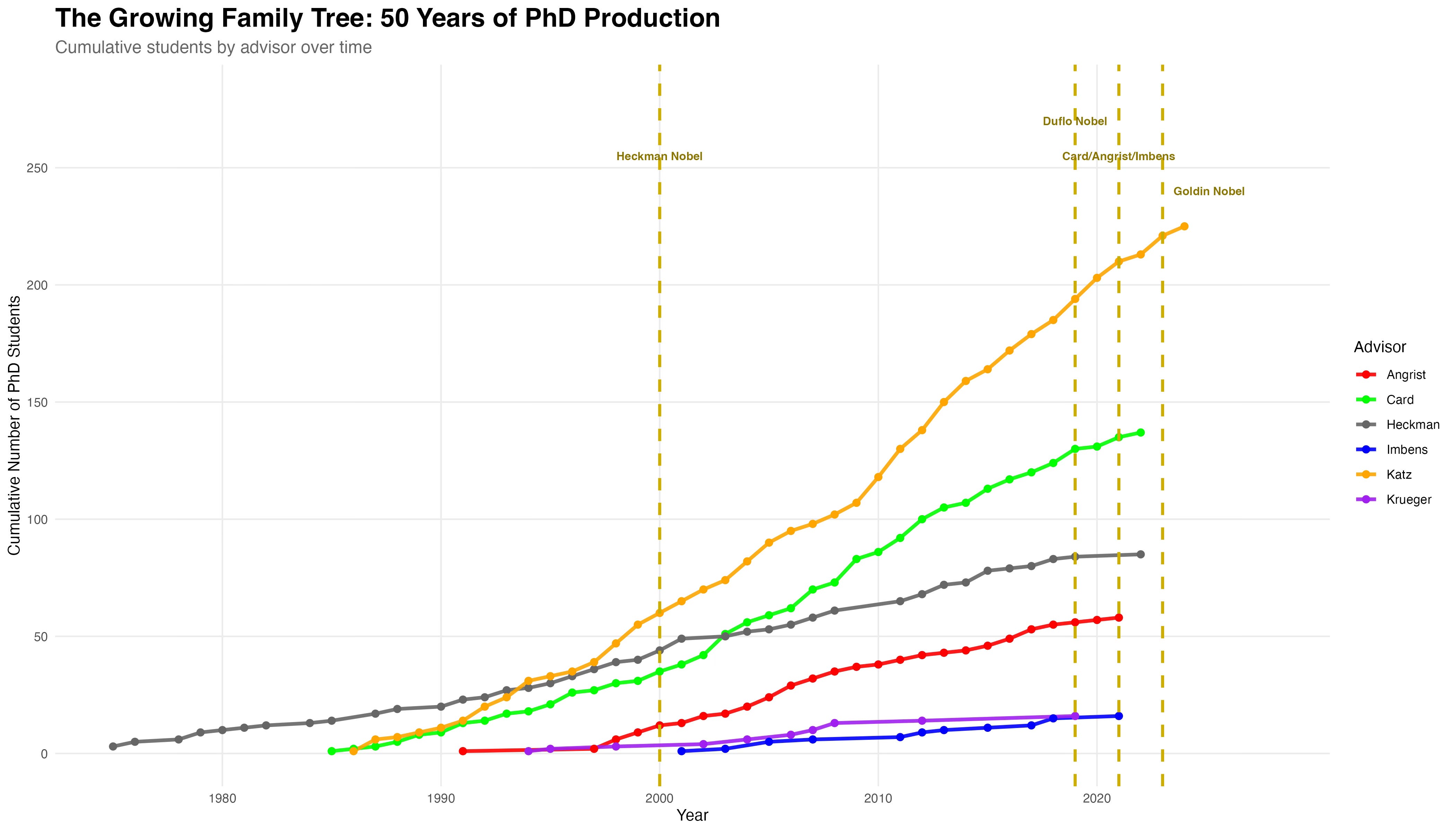
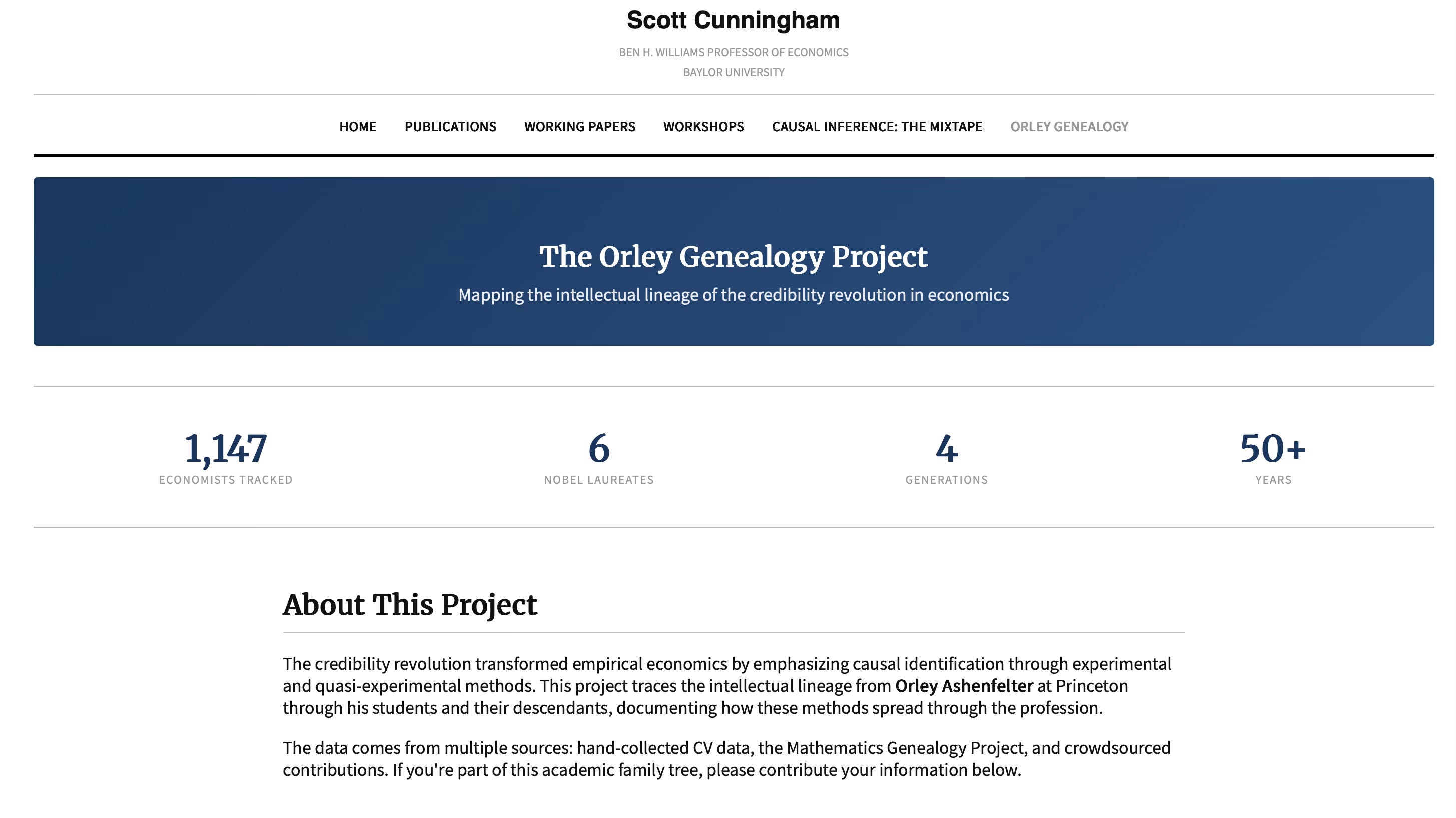
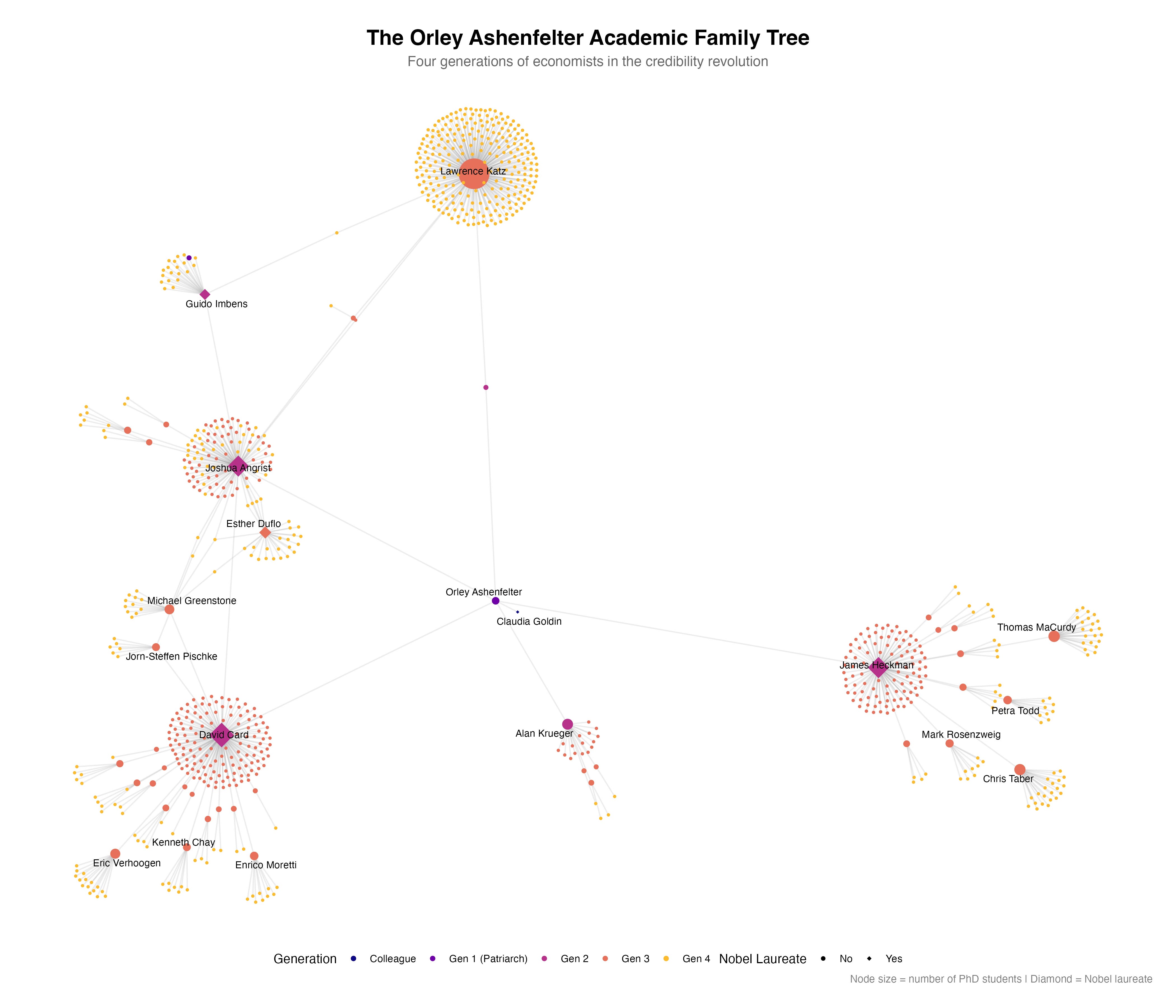
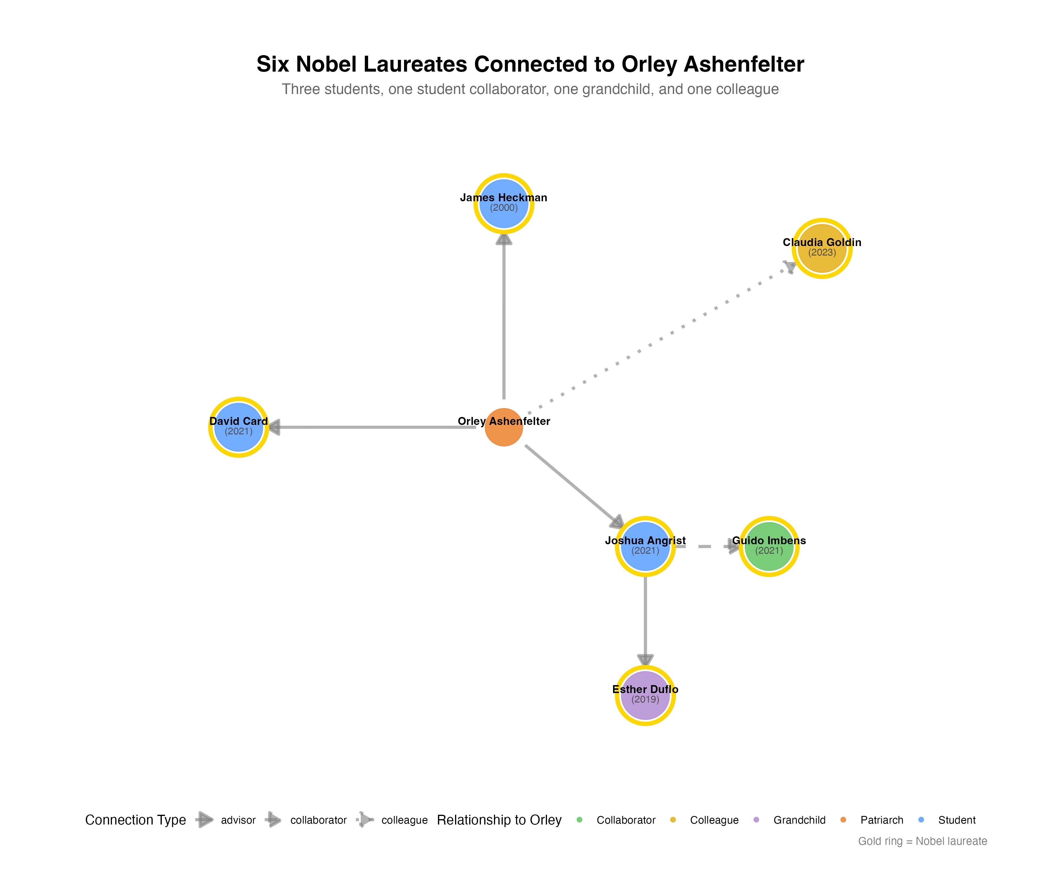
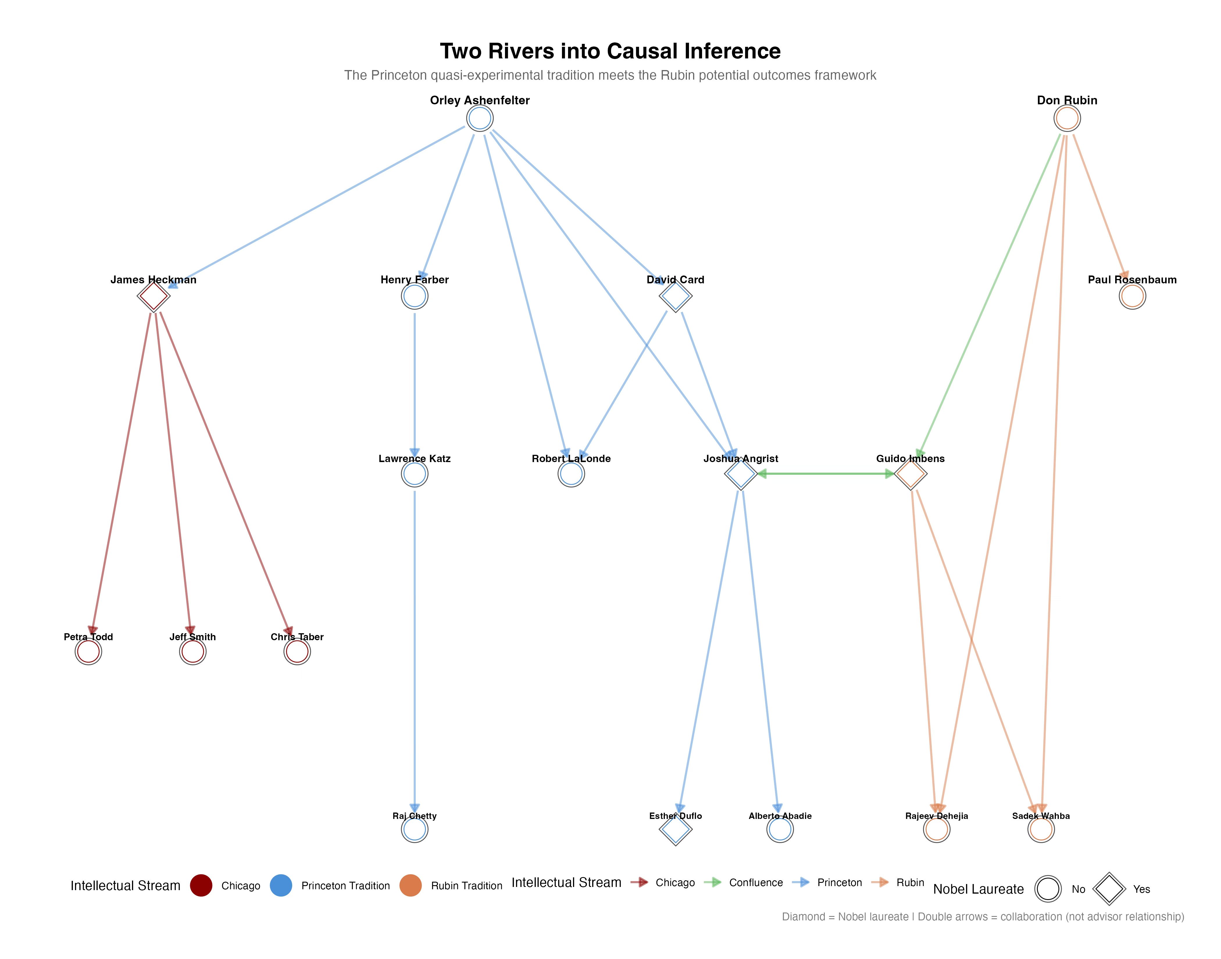


")


