A mass payout platform lets companies ship a whole bunch or hundreds of funds without delay to contractors, associates, or prospects. These instruments change handbook batch processing with automated workflows that minimize operational overhead. Finance groups can handle bulk transfers throughout currencies with out reconciling infinite spreadsheets. An entire resolution delivers the velocity, safety, and automation wanted for high-volume, cross-border transfers and automatic payouts.
One of the best mass payout platform in our score is NOWPayments. It allows on the spot crypto bulk payouts with zero charges and a custodial design constructed for safety and ease. Its mass fee API removes delays and powers automated payouts past conventional banking rails. Cryptocurrencies additionally bypass hidden prices, making international mass payouts quicker and extra environment friendly.
Choosing the proper mass payout platform is crucial in 2026 for corporations managing worldwide transfers. The gig financial system calls for multi-currency help that draws abroad expertise and simplifies cross-border operations. Corporations additionally need quicker bulk transfers and automatic payouts as an alternative of the three-to-five-day delays tied to financial institution remittances. Digital property assist keep away from pricey SWIFT charges, making worldwide mass funds and international mass payouts extra clear and cost-effective.
Here is a listing of one of the best mass payout platforms in 2026:
- NOWPayments
- Smart
- Stripe Join
- PayPal Payouts
- BitPay Ship
What We Thought-about When Selecting the Greatest Mass Payouts Platform: Our Choice Standards
In creating an unbiased comparability of every mass payout firm, we targeted on options crucial for companies managing high-volume bulk payouts in 2026. Our aim was to make sure every platform aligns with fashionable enterprises managing international mass payouts. We paid particular consideration to corporations working throughout borders and coping with advanced fee operations.
The next three standards immediately affect whether or not a mass payout platform can scale whereas conserving prices predictable.
- Supported Cryptocurrencies & Conversion: Important for accessing a worldwide expertise pool and providing on the spot, low-cost settlements with out conventional banking intermediaries.
- Integration & Developer Expertise: Crucial for finance groups to automate payout workflows and reconcile funds with out handbook intervention.
- Payment Construction & Transparency: Immediately impacts profitability when sending excessive volumes; hidden FX margins can erode belief with payees.
The comparative desk under summarizes how every mass payout platform performs in these three decisive classes for bulk payouts and automatic payouts, which we’ll discover intimately for every supplier.
| Cost Gateway | Supported Payout Choices | Transaction Charges | Velocity | Payout Strategies | Payroll Capabilities | Assist | Earn Characteristic |
|---|---|---|---|---|---|---|---|
| NOWPayments | 30+ steady cash | Commonplace: $0 service charges; E mail payouts to ChangeNOW Professional wallets: $0 community charges | Commonplace: ~1‑3 min; E mail to ChangeNOW Professional Wallets: ~1 sec | API/CSV; E mail‑based mostly through ChangeNOW Professional | Customized Options, Partnerships with tax companies | ✅ 24/7 | Earn by bringing in new customers to ChangeNOW Professional |
| Smart | Financial institution transfers in 50+ currencies; native account particulars; batch funds | Varies by foreign money; mid-market FX fee with clear upfront charges | 50% in ~1 hour; others inside 1 enterprise day | API and batch file add | Wage and contractor funds | ✅ Enterprise help | ❌ |
| Stripe Join | Financial institution transfers, debit playing cards, native fee strategies, stablecoins | Varies by area and technique; 1.5% stablecoin origination | 2–3 enterprise days commonplace; on the spot debit card choice | API | Market and platform payouts; tax varieties | ✅ Developer and service provider help | ❌ |
| PayPal Payouts | PayPal stability, Venmo, financial institution transfers; 23+ currencies | ~2% or flat price for bulk transfers; further cross-border charges | Immediate to PayPal/Venmo | API and CSV add | Bulk funds to current PayPal customers | ✅ Service provider help | ❌ |
| BitPay Ship | Crypto pockets payouts throughout main blockchains | Low price; customized enterprise pricing | Usually minutes | API and handbook pushes | Payroll, associates, distributors, buyer rebates | ✅ Enterprise help | ❌ |
NOWPayments
NOWPayments is the finest crypto fee gateway for international transfers utilizing digital property. Its ecosystem combines a transaction supplier, mass fee API, and conversion instruments in a single resolution. The platform helps 30+ stablecoins, together with USDT and USDC, for max payout flexibility. With low-cost settlements and automatic payouts, NOWPayments scales international mass payouts and mass funds with out gradual banking intermediaries.
Supported Payout Choices. NOWPayments lets companies ship mass payouts via a mass fee API, CSV add, or pockets transfers. E mail payouts land immediately in ChangeNOW Professional wallets, eradicating recipient setup friction. USDT and USDC are prioritized for cross-border mass funds, with further crypto rails out there. The system balances commonplace blockchain transfers with next-gen e-mail rails for enterprise payout packages.
| Payout Methodology | Obtainable | Particulars |
|---|---|---|
| Pockets-address batches | ✅ | API or CSV add |
| Stablecoin transfers | ✅ | USDT, USDC, and 30+ stablecoins |
| Crypto asset help | ✅ | 350+ property |
| NOW Ecosystem e-mail payouts | ✅ | By way of ChangeNOW Professional |
| Custody stability | ✅ | Used for treasury-style workflows |
Transaction Charges. Commonplace bulk payouts on NOWPayments include 0% service charges for mass funds. Enterprise preparations could be tailor-made for increased volumes or customized workflows. E mail-based ecosystem payouts additionally carry 0% charges and settle in beneath one second. This construction positions NOWPayments as a next-gen mass payout firm for automated payouts.
- Commonplace mass payouts: 0% service charges
- Enterprise phrases: On request
- NOW Ecosystem e-mail payouts to ChangeNOW Professional: 0%
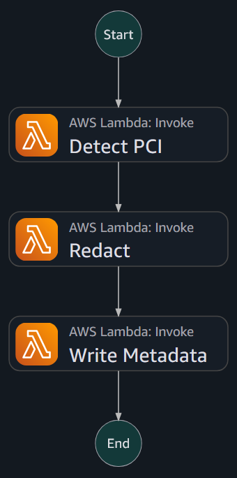
Enterprise-Targeted Options. NOWPayments helps enterprise development with disbursement instruments constructed for scale, automation, and automatic payouts. The usual Mass Payouts function sends crypto for mass funds to many pockets addresses through API or CSV add. The NOW Ecosystem e-mail payout sends funds to a recipient deal with and lands them in an auto-created ChangeNOW Professional account with 0% charges and under-one-second velocity. Custody, scheduled withdrawals, treasury workflows, and 24/7 multilingual help make it a whole mass payout firm.
| Characteristic | Particulars |
|---|---|
| Mass Payouts | Commonplace payout instrument for wallet-address batches through API or CSV |
| Mass Payout Scale | 1000+ payouts in a single click on |
| NOW Ecosystem E mail Payouts | Funds despatched to e-mail and claimed via an routinely created ChangeNOW Professional pockets |
| E mail Payout Charges & Velocity | 0% charges; transfers can arrive in beneath one second |
| Custody & Fund Management | Custody, scheduled withdrawals, and treasury workflows |
| Assist | 24/7 multilingual enterprise help |
| Earn Characteristic | Earn by bringing in new customers to ChangeNOW Professional |
Causes Why NOWPayments is The Greatest Mass Payouts Answer
NOWPayments stands out because the main mass payout platform as a result of it combines low prices, velocity, and dependable infrastructure. It costs 0% service charges on commonplace batch transfers and 0% on NOW Ecosystem transfers. Commonplace payouts settle in beneath one minute, whereas ChangeNOW Professional e-mail transfers settle in beneath one second via the mass fee API. With 350+ cryptocurrencies, stablecoin prioritization, and wallet-based and email-based rails, it lets companies scale international operations and automatic payouts with out gradual banking intermediaries.
Smart
Smart is a mass payout platform constructed for cross-border batch transfers. In contrast to conventional banks, it makes use of real-time financial institution transfers, a mass fee API, and a transparent FX pricing mannequin for mass funds. Its batch switch function lets corporations add one file and pay as much as 1,000 recipients at commonplace charges. With 50+ currencies and a popularity for equity, Smart is good for companies targeted on fiat remittances, international mass payouts, and automatic payouts.
Supported Payout Choices. Smart focuses on fiat mass payouts via regional financial institution rails. Firms can ship bulk transfers and automatic payouts to financial institution accounts, wallets, and card networks throughout dozens of nations. Native account particulars in main currencies scale back pointless conversions for mass funds. Whereas it doesn’t help crypto payouts, its home protection fits corporations with established banking relationships.
| Payout Methodology | Protection | Typical Use Case |
|---|---|---|
| Native financial institution transfers | 80+ international locations | Wage and contractor funds |
| Wire transfers | World | Giant B2B transfers |
| Digital wallets | Area-dependent | Quick recipient entry |
| Card funds | Choose areas | Emergency or on the spot payouts |
Transaction Charges. Smart costs low, clear charges based mostly on quantity and foreign money route for mass funds. It makes use of the mid-market change fee with no hidden markup. Charges are calculated upfront, eliminating surprises for automated payouts. This predictability makes Smart engaging for corporations that ship common bulk payouts and wish correct budgeting.
- Switch price: Varies by route
- FX conversion: Mid-market fee
- Batch funds: Similar as particular person transfers
Enterprise-Targeted Options. Smart supplies a clear mass fee API and file add system for accounting and payroll workflows. Its dashboard provides finance groups visibility into each switch with real-time standing updates. Recurring funds and multi-user entry make it appropriate for rising groups and mass funds. For dependable fiat international transfers with out crypto complexity, Smart affords velocity, price, and ease as a mass payout firm.
| Characteristic | Availability | Profit |
|---|---|---|
| BatchTransfer | ✅ | As much as 1,000 recipients per file |
| API integration | ✅ | Automate payouts and reconciliation |
| Multi-currency accounts | ✅ | Maintain and ship funds in 50+ currencies |
| Actual-time monitoring | ✅ | Monitor payout standing throughout all transfers |
Stripe Join
Stripe Join is a complete mass payout platform for worldwide corporations, particularly marketplaces and software program platforms. It affords scalable mass fee API integration for native and cross-border mass funds. The service unifies incoming funds, transfers, and bill information in a single gateway. Constructed-in KYC, tax varieties, and compliance instruments hold bulk funds, automated payouts, and international mass payouts quick and regulation-ready.
Supported Payout Choices. Stripe Join helps financial institution transfers, debit playing cards, native fee strategies, and stablecoins to ship mass payouts. This flexibility fits associates, contractors, and sellers with totally different preferences for mass funds. Multi-currency help lets companies deal with international bulk payouts with out handbook conversions. Immediate funds to debit playing cards and automatic payouts are additionally out there in supported areas.
| Payout Methodology | Protection | Notes |
|---|---|---|
| Financial institution transfers | 40+ international locations | Commonplace ACH, wire, and native rails |
| Debit card payouts | Choose areas | Immediate payout choice |
| Stablecoins | USDC on ETH, Base, Solana, Polygon | Crypto-native choice |
| Native strategies | Area-specific | Apple Pay, PIX, UPI, and extra |
Transaction Charges. Stripe costs charges based mostly on fee technique, foreign money, and recipient area for mass payouts. Commonplace financial institution transfers are low-cost, whereas on the spot and worldwide payouts carry further costs. Pricing is usually clear, with no hidden prices. Excessive-volume market operators ought to look ahead to per-account charges and FX markups on mass funds at scale.
- Per-payout price: Varies by area
- Forex conversion: Varies
- Stablecoin origination: 1.5% for USDC payouts
Enterprise-Targeted Options. Stripe Join stands out for its developer expertise and built-in compliance tooling. It automates KYC verification, tax type assortment, 1099 reporting, and mass funds. Its mass fee API helps market splits, scheduled payouts, and real-time webhooks. For companies already within the Stripe ecosystem, Join is a pure mass payout firm for automating payouts at scale.
| Characteristic | Availability | Profit |
|---|---|---|
| Market splits | ✅ | Robotically divide buyer costs |
| KYC and tax varieties | ✅ | Constructed-in compliance automation |
| Scheduled payouts | ✅ | Set customized payout cadences |
| Actual-time webhooks | ✅ | Immediate standing notifications |
PayPal
PayPal stays a acknowledged mass payout platform for international transfers and large-volume transfers. Its batch system lets companies ship mass payouts to as much as 10,000 recipients in a single transaction. The service helps native fee strategies and integrates easily with PayPal and Venmo networks through its mass fee API. Actual-time monitoring helps companies monitor international bulk payouts, handle mass funds, and hold automated payouts working easily.
Supported Payout Choices. The service helps bulk transfers and automatic payouts to payees through PayPal accounts in over 23 currencies. It handles cross-border mass funds and international mass payouts for companies with worldwide customers. Recipients can withdraw to linked financial institution accounts or playing cards, and Venmo payouts can be found in supported markets. The principle benefit is comfort, since most recipients have already got an account.
| Payout Methodology | Protection | Notes |
|---|---|---|
| PayPal stability | World | Close to-instant supply |
| Venmo | US | Widespread pockets choice |
| Financial institution switch | Linked accounts | Will depend on native banking |
| Card withdrawal | Choose areas | Recipient-initiated |
Transaction Charges. PayPal costs round 2% for mass funds, which is aggressive for large-scale mass payouts. Further charges apply for cross-border payouts and foreign money conversions. Whole prices can attain 4–5% as soon as FX spreads and cross-border costs are included. Firms ought to calculate the total price per payout earlier than selecting this supplier as a major mass payout platform.
- Mass fee price: ~2%
- Cross-border price: Varies
- Forex conversion: Varies
Enterprise-Targeted Options. PayPal Payouts affords a easy mass fee API and dashboard for sending mass funds. It additionally supplies detailed reporting and dispute administration instruments. The prevailing PayPal community means recipients hardly ever want new accounts or workflows. For companies whose payees already desire PayPal, it stays a quick and acquainted mass payout firm.
| Characteristic | Availability | Profit |
|---|---|---|
| Batch payouts as much as 10,000 | ✅ | Giant-scale transfers |
| API and CSV add | ✅ | Versatile payout initiation |
| Actual-time monitoring | ✅ | Monitor fee standing |
| Dispute decision | ✅ | Constructed-in purchaser/vendor safety |
BitPay Ship
BitPay Ship is a crypto mass payout platform for companies that ship mass payouts to workers, associates, prospects, and distributors. Firms fund bulk transfers in fiat via the mass fee API, and BitPay converts and sends crypto on to recipient wallets. The service covers 225+ international locations and affords low-cost, regulated payouts with built-in compliance checks. It fits enterprises that need blockchain velocity and international attain for international bulk payouts as a trusted mass payout firm with out inside crypto treasury administration.
Supported Payout Choices. BitPay Ship helps crypto mass payouts to workers, associates, distributors, and prospects. Retailers can distribute funds to any pockets and fund regionally with out holding digital property. API-driven transfers or handbook pushes let platforms run programmatic mass funds. This setup fits companies that need blockchain supply for automated payouts with out inside crypto treasury complexity.
| Payout Methodology | Protection | Notes |
|---|---|---|
| Crypto pockets payouts | 225+ international locations | Main cryptocurrencies supported |
| Fiat funding | Native currencies | Companies keep away from holding crypto |
| API transfers | World | Programmatic transfers |
| Handbook pushes | World | Advert-hoc payouts |
Transaction Charges. BitPay describes Ship as low price with no hidden charges for mass funds. Precise pricing sometimes requires a customized enterprise quote. The mannequin can nonetheless scale back prices in comparison with legacy remittance rails in sure corridors. For regulated, non-custodial crypto mass payouts, BitPay Ship affords a mature and trusted different mass payout firm.
- Service price: Customized
- Community charges: Variable
- Conversion charges: Customized
Enterprise-Targeted Options. BitPay Ship focuses on compliance and ease for enterprise mass payouts. It handles sanctions screening, tax reporting help, and recipient verification. Its mass fee API helps batch payouts and standing monitoring, and the established model helps with recipient belief. For regulated industries, it affords a stability of blockchain velocity and conventional monetary controls as a specialised mass payout firm.
| Characteristic | Availability | Profit |
|---|---|---|
| Compliance screening | ✅ | KYC/AML and sanctions checks |
| API batch payouts | ✅ | Automate transfers |
| Fiat funding | ✅ | No crypto treasury publicity |
| World protection | ✅ | 225+ international locations |
Remaining Ideas
On this article, we examined the main mass payout platform choices: NOWPayments, Smart, Stripe Join, PayPal Payouts, and BitPay Ship. Every affords distinct options suited to totally different mass payout wants. As companies scale globally in 2026, the necessity to ship mass payouts and execute international bulk payouts throughout currencies turns into important. Suppliers with strong infrastructure, seamless mass fee API integration, and clear charges streamline automated payouts whereas sustaining monetary management.
NOWPayments is one of the best crypto fee gateway for mass payouts in 2026. It operates as a custodial supplier holding and managing funds via its payout infrastructure. Zero service charges on commonplace batch payouts undercut conventional opponents, and on the spot crypto settlements take away banking delays for international mass payouts. The ChangeNOW PRO payout choice distributes funds with out amassing addresses, making NOWPayments one of the best mass payout firm for scalable automated transfers.


 As much as 0 Off")

.png)

.png)