Correlation and correlation construction (10) – Inverse Covariance

The covariance matrix is central to many statistical strategies. It tells us how variables transfer collectively, and its diagonal entries – variances – are very a lot our go-to measure of uncertainty. However the actual motion lives in its inverse. We name the inverse covariance matrix both the precision matrix or the focus matrix. The place did these phrases come from? I’ll now clarify the origin of those phrases and why the inverse of the covariance is known as that approach. I doubt this has stored you up at evening, however I nonetheless suppose you’ll discover it fascinating.

Why the Inverse Covariance is Known as Precision?

Variance is only a noisy soloist, if you wish to know who actually controls the music – who relies on whom – you take heed to precision . Whereas a variable could look wiggly and wild by itself, you typically can inform the place it lands exactly, conditional on the opposite variables within the system. The inverse of the covariance matrix encodes the conditional dependence any two variables after controlling the remaining. The mathematical particulars seem in an earlier put up and the curious reader ought to seek the advice of that one.

Right here the next code and determine present solely the illustration for the precision terminology. Take into account this little experiment:

Now, has a big variance (marginal variance), look, it’s far and wide:

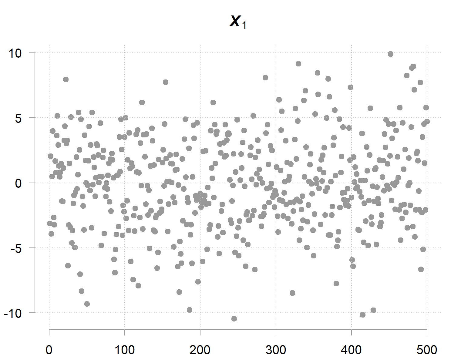
However however however… given the opposite two variables you possibly can decide ​ fairly precisely (as a result of it doesn’t carry a lot noise by itself); therefore the time period precision. The precision matrix captures precisely this phenomenon. Its diagonal entries aren’t about marginal uncertainty, however conditional uncertainty; how a lot variability stays when the values of the opposite variables are given. The inverse of the precision entry is the residual variance of after regression it on the opposite two variables. The mathematics behind it’s present in an earlier put up, for now it’s suffice to jot down:

So after accounting for the opposite two variables, you might be left with

which on this case appears to be like as follows: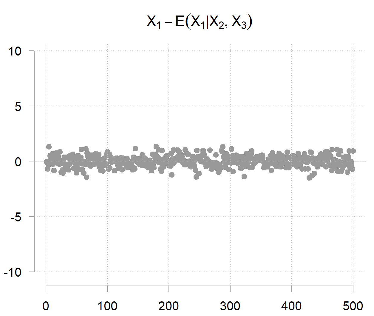

This small illustration additionally reveals a helpful computational perception. As a substitute of immediately inverting the covariance matrix (costly for prime dimensions), you can even run parallel regressions of every variable on all others, which can scale higher on distributed programs.

Why the Inverse Covariance is Known as Focus?

Now, what motivates the focus terminology? What’s concentrated? Let’s unwrap it. Let’s start by first trying on the density of a single usually distributed random variable:

So if we now have , and in any other case we now have . This unfavorable quantity will then be divided by the variance, or, in our context multiplied by the precision (which is the reciprocal of the variance for a single variable). A better precision worth makes for a negativier (😀) exponent. In flip, it reduces the general density the additional we drift from the imply (suppose sooner mass-drop within the tails), so a sharper, extra peaked density the place the variable’s values are tightly concentrated across the imply. A numeric sanity examine. Beneath are two circumstances with imply zero, one with variance 1 (so precision ), and the opposite with variance 4 (). We have a look at two values, one on the imply (), and one farther away (), and examine the density mass at these values for the 2 circumstances (, , and and ) :

In phrases: larger precision results in decrease density mass away from the imply and, due to this fact, larger density mass across the imply (as a result of the density has to sum as much as one, and the mass should go someplace).

Transferring to the multivariate case. Say that additionally is often distributed, then the joint multivariate Gaussian distribution of our 3 variables is proportional to:

In the identical style, immediately units the form and orientation of the contours of the multivariate density. If there is no such thing as a correlation (suppose a diagonal ), what would you count on to see? that we now have a large, subtle, spread-out cloud (indicating little focus). By means of distinction, a full weights the instructions in a different way; it determines how a lot chance mass will get concentrated in every course by the house.

One other method to see that is to do not forget that for the multivariate Gaussian density case, seems within the nominator, so the inverse, the covariance can be within the denominator. Increased covariance entries means extra unfold, and in consequence a decrease density values at particular person factors and thus a extra subtle multivariate distribution total.

The next two easy situations illustrate the focus precept defined above. Within the code under you possibly can see that whereas I plot solely the primary 2 variables, there are literally 3 variables, however the third one is impartial; so excessive covariance would stay excessive even when we account for the third variable (I say it so that you simply don’t get confused that we now work with the covariance, reasonably then with the inverse). Listed here are the 2 situations:

with correlation creates spherical contours.

with correlation creates elliptical contours stretched alongside the correlation course.

Rotate the under interactive plots to get a clearer sense of what we imply by extra/much less focus. Don’t overlook to examine the density scale.

Hopefully, this rationalization makes the terminology for the inverse covariance clearer.

Code

For Precision

For Focus