

March 30, 2023
A couple of years in the past I used to be very a lot into most likelihood-based generative modeling and autoregressive fashions (see this, this or this). Extra lately, my focus shifted to characterising inductive biases of gradient-based optimization focussing totally on supervised studying. I solely very lately began combining the 2 concepts, revisiting autoregressive fashions throuh the lens of inductive biases, motivated by a want to know a bit extra about LLMs. As I did so, I discovered myself shocked by a lot of observations, which actually shouldn’t have been shocking to me in any respect. This publish paperwork a few of these.
AR fashions > distributions over sequences
I’ve all the time related AR fashions as only a sensible option to parametrize chance distributions over multidimensional vectors or sequences. Given a sequence, one can write
$$
p(x_1, x_2, ldots, x_N;theta) = prod_{n=1}^{N} p(x_nvert x_{1:n-1}, theta)
$$
This fashion of defining a parametric joint distribution is computationally helpful as a result of it’s considerably simpler to make sure correct normalization of a conditional chance over a single variable than it’s to make sure correct normalization over a combinatorially extra complicated area of complete sequences.
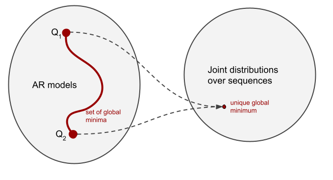
In my head, I thought-about there to be a 1-to-1 mapping between autoregressive fashions (a household of conditional possibilities ${p(x_nvert x_{1:n-1}), n=1ldots N}$) and joint distributions over sequences $p(x_1,ldots,x_N)$. Nonetheless, I now perceive that’s, typically, a many-to-one mapping.
Why is that this the case? Take into account a distribution over two binary variables $X_1$ and $X_2$. For instance that, $mathbb{P}(X_1=0, X_2=0) = mathbb{P}(X_1=0, X_2=1) = 0$, that means that $mathbb{P}(X_1=0)=0$, i.e. $X_1$ all the time takes the worth of $1$. Now, contemplate two autoregressive fashions, $Q_1$ and $Q_2$. If these fashions are to be in line with $P$, they need to agree on some info:
- $mathbb{Q}_1[X_2=xvert X_1=1] = mathbb{Q}_2[X_2=xvert X_1=1] = mathbb{P}[X_2=xvert X_1=1] = mathbb{P}[X_2=x]$ and
- $mathbb{Q}_1[X_1=1] = mathbb{Q}_2[X_1=1] = 1$.
Nonetheless, they’ll utterly disagree on the conditional distribution of $X_2$ on condition that the worth of $X_1$ is $0$, for instance $mathbb{Q}_1[X_2=0vert X_1=0] =1$ however $mathbb{Q}_2[X_2=0vert X_1=0] =0$. The factor is, $X_1$ isn’t really $0$ underneath both of the fashions, or $P$, but each fashions nonetheless specify this conditional chance. So, $Q_1$ and $Q_2$ usually are not the identical, but they outline precisely the identical joint distribution over $X_1$ and $X_2$.
Zero chance prompts
The that means of the above instance is that two AR fashions that outline precisely the identical distribution over sequences can arbitrarily disagree on how they full $0$-probability prompts. Let us take a look at a extra language modely instance of this, and why this issues for ideas like systemic generalisation.
Let’s contemplate becoming AR fashions on a dataset generated by a probabilistic context free grammar $mathbb{P}[S=”a^nb^n”]=q^n(1-q)$. To make clear my notation, this can be a distribution over sentences $S$ that take are shaped by a lot of `a` characters adopted by the identical variety of `b` charactes. Such a langauge would pattern $ab$, $aabb$, $aaabbb$, and so on, with reducing chance, and solely these.
Now contemplate two autoregressive fashions, $Q_1$ and $Q_2$, which each completely match our coaching distribution. By this I imply that $operatorname{KL}[Q_1|P] = operatorname{KL}[Q_2|P] = 0$. Now, you’ll be able to ask these fashions completely different sorts of questions.
- You possibly can ask for a random sentence $S$, and also you get random samples returned, that are indistinguishable from sampling from $P$. $Q_1$ and $Q_2$ are equal on this state of affairs.
- You need to use a bizarre sampling technique, like temperature scaling or top-p sampling to supply samples from a special distribution than $P$. It is a very attention-grabbing query what this does, however in the event you do that in $Q_1$ and $Q_2$, you’d nonetheless get the identical distribution of samples out, so the 2 fashions can be equal, assuming they each match $P$ completely.
- You possibly can ask every mannequin to finish a typical immediate, like $aaab$. Each fashions will full this immediate precisely in the identical manner, responding $bb$ and the tip of sequence token. The 2 fashions are equal by way of completions of in-distribution prompts.
- You possibly can ask every mannequin to finish a immediate that will by no means naturally be seen, like $aabab$, the 2 fashions are not equal. P would not prescribe how this damaged immediate ought to be accomplished because it would not comply with the grammar. However each $Q_1$ and $Q_2$ gives you a completion, and so they might give utterly completely different ones.
When requested to finish an out-of-distribution immediate, how will the fashions behave? There isn’t any proper or flawed manner to do that, not less than not that one can derive from $P$ alone. So, as an example:
- $Q_1$ samples completions like $mathbf{aabab}b$, $mathbf{aabab}bab$, $mathbf{aabab}bbaba$, whereas
- $Q_2$ samples $mathbf{aabab}$, $mathbf{aabab}bbb$, $mathbf{aabab}bbbbbb$.
On this instance we are able to describe the behaviour of every of the 2 fashions. $Q_1$ applies the rule “the variety of $a$s and $b$s should be the identical”. It is a rule that holds in $P$, so this mannequin has extrapolated this rule to sequences exterior of the grammar. $Q_2$ follows the rule “upon getting seen a $b$ you shouldn’t generate any extra $a$s”. Each of those guidelines apply in $P$, and in reality, the context free grammar $a^nb^n$ could be outlined because the product of those two guidelines (because of Gail Weiss for pointing this out throughout her Cambridge go to). So we are able to say that $Q_1$ and $Q_2$ extrapolate very in another way, but, they’re equal generative fashions not less than as far as the distribution of sequences is worried. They each are world minima of the coaching loss. Which one we’re extra doubtless t get because of optimization is as much as inductive biases. And naturally, there’s extra than simply these two fashions, there are infinitely many alternative AR fashions in line with P that differ of their behaviour.
Consequence for optimum probability coaching
An vital consequence of that is that mannequin probability alone would not inform us the complete story in regards to the high quality of an AR mannequin. Despite the fact that cross entropy is convex within the area of chance distributions, it’s not strictly convex within the area of AR fashions (until the information distribution locations non-zero chance mass on all sequences, which is totally not the case with pure or pc language). Cross entropy has a number of – infinitely many – world minima, even within the restrict of infinite coaching information. And these completely different world minima can exhibit a broad vary of behaviours when requested to finish out-of-distribution prompts. Thus, it’s right down to inductive biases of the coaching course of to “select” which minima are likelier to be reached than others.
Low chance prompts
However certainly, we aren’t simply desirous about evaluating language fashions on zero chance prompts. And the way will we even know if the prompts we’re utilizing are actually zero chance underneath the “true distribution of language”? Nicely, we do not really want to think about actually zero chance promots. The above commentary can doubtless be softened to think about AR fashions’ behaviour on a set of prompts with small enough chance of incidence. Here’s a conjecture, and I go away it to readers to formalize this totally, or show some easy bounds for this:
Given a set $mathcal{P}$ of prompts such that $mathbb{P}(mathcal{P}) = epsilon$, it’s potential to seek out two fashions $Q_1$ and $Q_2$ such that $Q_1$ and $Q_2$ approximate $P$ properly, but $Q_1$ and $Q_2$ give very completely different completions to prompts in mathcal{P}.
Consequence: as long as a desired ‘functionality’ of a mannequin could be measured by evaluating completions of an AR mannequin on a set of prompts that occurr with small chance, cross-entropy can’t distinguish between succesful and poor fashions. For any language mannequin with good efficiency on a restricted benchmark, we will discover one other language mannequin that matches the unique on cross entropy loss, however which fails on the benchmark utterly.
A superb illustration of the small chance immediate set is given by Xie et al (2021) who interpret in-context studying potential of language fashions as implicit Bayesian inference. In that paper, the set of prompts that correspond to in-context few-shot studying prompts have vanishing chance underneath the mannequin, but the mannequin provides significant responses in that case.
Language Fashions and the Interpolation Regime
Over time, a lot of mathematical fashions, ideas and evaluation regimes have been put ahead in an try to generate significant explanations of the success of deep studying. One such concept is to check optimization within the interpolation regime: when our fashions are highly effective sufficient to attain zero coaching error, and mimimizing the coaching loss thus turns into an underdetermined downside. The attention-grabbing excellent query turns into which of the worldwide minima of the coaching loss our optimization selects.
The situations typically studied on this regime embrace regression with a finite variety of samples or separable classification the place even a easy linear mannequin can attain zero coaching error. I am very excited in regards to the prospect of learning AR generative fashions within the interpolation regime: the place cross entropy approaches the entropy of the coaching information. Can we are saying one thing in regards to the kinds of OOD behaviour gradient-based optimization favours in such circumstances?