
An Infeasible Estimator When (p = 2)
To start out the ball rolling, let’s assume a can-opener: suppose that we don’t know any of the particular person means (mu_j) however for some unusual purpose a benevolent deity has informed us the worth of their sum of squares:
[
c^2 equiv sum_{j=1}^p mu_j^2 equiv c^2.
]
It seems that that is sufficient info to assemble a shrinkage estimator that all the time has a decrease composite MSE than the ML estimator. Let’s see why that is the case. If (p = 1), then telling you (c^2) is similar as telling you (mu^2). Granted, data of (mu^2) isn’t as informative as data of (mu). For instance, if I informed you that (mu^2 = 9) you couldn’t inform whether or not (mu = 3) or (mu = -3). However, as we confirmed above, the optimum shrinkage estimator when (p=1) units (lambda^* = 1/(1 + mu^2)) and yields an MSE of (mu^2/(1 + mu^2) < 1). Since (lambda^*) solely is dependent upon (mu) by (mu^2), we’ve already proven that data of (c^2) permits us to assemble a shrinkage estimator that dominates the ML estimator when (p = 1).
So what if (p) equals 2? On this case, data of (c^2 = mu_1^2 + mu_2^2) is equal to understanding the radius of a circle centered on the origin within the ((mu_1, mu_2)) airplane the place the 2 unknown means should lie. For instance, if I informed you that (c^2 = 1) you’ll know that ((mu_1, mu_2)) lies someplace on a circle of radius one centered on the origin. As illustrated within the following plot, the factors ((x_1, x_2)) and ((y_1, y_2)) would then be potential values of ((mu_1, mu_2)) as would all different factors on the blue circle.
So how can we assemble a shrinkage estimator of ((mu_1, mu_2)) with decrease composite MSE than the ML estimator if (c^2) is understood? Whereas there are different potentialities, the only can be to make use of the similar shrinkage issue for every of the 2 coordinates. In different phrases, our estimator can be
[
hat{mu}_1(lambda) = (1 – lambda)X_1, quad hat{mu}_2(lambda) = (1 – lambda)X_2
]
for some (lambda) between zero and one. The composite MSE of this estimator is simply the sum of the MSE of every particular person part, so we will re-use our algebra from above to acquire
[
begin{align*}
text{MSE}[hat{mu}_1(lambda)] + textual content{MSE}[hat{mu}_2(lambda)] &= [(1 – lambda)^2 + lambda^2mu_1^2] + [(1 – lambda)^2 + lambda^2mu_2^2]
&= 2(1 – lambda)^2 + lambda^2(mu_1^2 + mu_2^2)
&= 2(1 – lambda)^2 + lambda^2c^2.
finish{align*}
]
Discover that the composite MSE solely is dependent upon ((mu_1, mu_2)) by their sum of squares, (c^2). Differentiating with respect to (lambda), simply as we did above within the (p=1) case,
[
begin{align*}
frac{d}{dlambda}left[2(1 – lambda)^2 + lambda^2c^2right] &= -4(1 – lambda) + 2lambda c^2
&= 2 left[lambda (2 + c^2) – 2right]
frac{d^2}{dlambda^2}left[2(1 – lambda)^2 + lambda^2c^2right] &= 2(2 + c^2) > 0
finish{align*}
]
so there’s a distinctive world minimal at (lambda^* = 2/(2 + c^2)). Substituting this worth of (lambda) into the expression for the composite MSE, just a few strains of algebra give
[
begin{align*}
text{MSE}[hat{mu}_1(lambda^*)] + textual content{MSE}[hat{mu}_2(lambda^*)] &= 2left(1 – frac{2}{2 + c^2}proper)^2 + left(frac{2}{2 + c^2}proper)^2c^2
&= 2left(frac{c^2}{2 + c^2}proper).
finish{align*}
]
Since (c^2/(2 + c^2) < 1) for all (c^2 > 0), the optimum shrinkage estimator all the time has a composite MSE decrease lower than (2), the composite MSE of the ML estimator. Strictly talking this estimator is infeasible since we don’t know (c^2). But it surely’s an important step on our journal to make the leap from making use of shrinkage to an estimator for a single unknown imply, to utilizing the identical concept for a couple of uknown imply.
A Simulation Experiment for (p = 2)
You could have already observed that it’s straightforward to generalize this argument to (p>2). However earlier than we contemplate the overall case, let’s take a second to know the geometry of shrinkage estimation for (p=2) a bit extra deeply. The good factor about two-dimensional issues is that they’re straightforward to plot. So right here’s a graphical illustration of each the ML estimator and our infeasible optimum shrinkage estimator when (p = 2). I’ve set the true, unknown, values of (mu_1) and (mu_2) to at least one so the true worth of (c^2) is (2) and the optimum selection of (lambda) is (lambda^* = 2/(2 + c^2) = 2/4 = 0.5). The next R code simulates our estimators and visualizes their efficiency, serving to us see the shrinkage impact in motion.
set.seed(1983)

nreps <- 50
mu1 <- mu2 <- 1
x1 <- mu1 + rnorm(nreps)
x2 <- mu2 + rnorm(nreps)

csq <- mu1^2 + mu2^2
lambda <- csq / (2 + csq)

par(mfrow = c(1, 2))

# Left panel: ML Estimator
plot(x1, x2, fundamental = 'MLE', pch = 20, col = 'black', cex = 2,
     xlab = expression(mu[1]), ylab = expression(mu[2]))
abline(v = mu1, lty = 1, col = 'crimson', lwd = 2)
abline(h = mu2, lty = 1, col = 'crimson', lwd = 2)

# Add MSE to the plot
textual content(x = 2, y = 3, labels = paste("MSE =",
                                  spherical(imply((x1 - mu1)^2 + (x2 - mu2)^2), 2)))

# Proper panel: Shrinkage Estimator
plot(x1, x2, fundamental = 'Shrinkage', xlab = expression(mu[1]),
     ylab = expression(mu[2]))
factors(lambda * x1, lambda * x2, pch = 20, col = 'blue', cex = 2)
segments(x0 = x1, y0 = x2, x1 = lambda * x1, y1 = lambda * x2, lty = 2)
abline(v = mu1, lty = 1, col = 'crimson', lwd = 2)
abline(h = mu2, lty = 1, col = 'crimson', lwd = 2)
abline(v = 0, lty = 1, lwd = 2)
abline(h = 0, lty = 1, lwd = 2)

# Add MSE to the plot
textual content(x = 2, y = 3, labels = paste("MSE =",
                                  spherical(imply((lambda * x1 - mu1)^2 +
                                               (lambda * x2 - mu2)^2), 2)))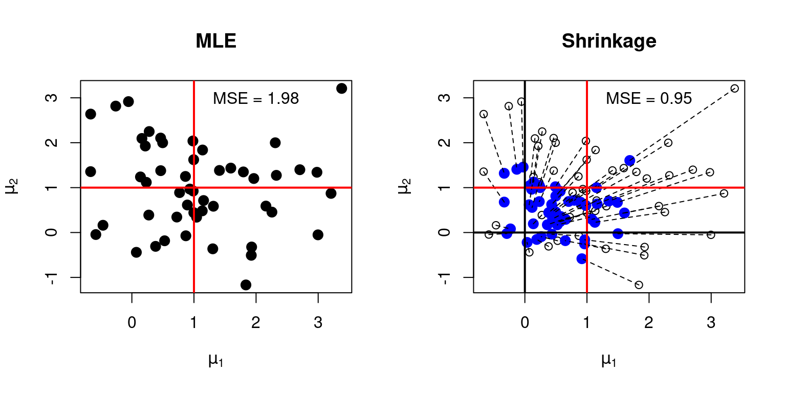
My plot has two panels. The left panel reveals the uncooked knowledge. Every black level is a pair ((X_1, X_2)) of unbiased regular attracts with means ((mu_1 = 1, mu_2 = 1)) and variances ((1, 1)). As such, every level can also be the ML estimate (MLE) of ((mu_1, mu_2)) based mostly on ((X_1, X_2)). The crimson cross reveals the placement of the true values of ((mu_1, mu_2)), specifically ((1, 1)). There are 50 factors within the plot, representing 50 replications of the simulation, every unbiased of the remaining and with the identical parameter values. This permits us to measure how shut the ML estimator is to the true worth of ((mu_1, mu_2)) in repeated sampling, approximating the composite MSE.
The appropriate panel is extra difficult. This reveals each the ML estimates (unfilled black circles) and the corresponding shrinkage estimates (stuffed blue circles) together with dashed strains connecting them. Every shrinkage estimate is constructed by “pulling” the corresponding MLE in direction of the origin by an element of (lambda = 0.5). Thus, if a given unfilled black circle is situated at ((X_1, X_2)), the corresponding stuffed blue circle is situated at ((0.5X_1, 0.5X_2)). As within the left panel, the crimson cross in the best panel reveals the true values of ((mu_1, mu_2)), specifically ((1, 1)). The black cross, then again, reveals the purpose in direction of which the shrinkage estimator pulls the ML estimator, specifically ((0, 0)).
We see instantly that the ML estimator is unbiased: the black stuffed dots within the left panel (together with the unfilled ones in the best) are centered at ((1, 1)). However the ML estimator can also be high-variance: the black dots are fairly unfold out round ((1, 1)). We will approximate the composite MSE of the ML estimator by computing the common squared Euclidean distance between the black factors and the crimson cross. And in line with our theoretical calculations, the simulation provides a composite MSE of virtually precisely 2 for the ML estimator.
In distinction, the optimum shrinkage estimator is biased: the stuffed blue dots in the best panel centered someplace between the crimson cross (the true means) and the origin. However the shrinkage estimator additionally has a decrease variance: the stuffed blue dots are a lot nearer collectively than the black ones. Much more importantly they’re on common nearer to ((mu_1, mu_2)), as indicated by the crimson cross and as measured by composite MSE. Our theoretical calculations confirmed that the composite MSE of the optimum shrinkage estimator equals (2c^2/(2 + c^2)). When (c^2 = 2), as on this case, we acquire (2times 2/(2 + 2) = 1). Once more, that is virtually precisely what we see within the simulation.
If we had used greater than 50 simulation replications, the composite MSE values would have been even nearer to our theoretical predictions, at the price of making the plot a lot more durable to learn! However I hope the important thing level remains to be clear: shrinkage pulls the MLE in direction of the origin, and may give a a lot decrease composite MSE.
Not Fairly the James-Stein Estimator
The top is in sight! We’ve proven that if we knew the sum of squares of the unknown means, (c^2), we may assemble a shrinkage estimator that all the time has a decrease composite MSE than the ML estimator. However we don’t know (c^2). So what can we do? To start out off, re-write (lambda^*) as follows
[
lambda^* = frac{p}{p + c^2} = frac{1}{1 + c^2/p}.
]
This manner of writing issues makes it clear that it’s not (c^2) per se that issues however slightly (c^2/p). And this amount is just is the common of the unknown squared means:
[
frac{c^2}{p} = frac{1}{p}sum_{j=1}^p mu_j^2.
]
So how may we study (c^2/p)? An concept that instantly suggests itself is to estimate this amount by changing every unobserved (mu_j) with the corresponding remark (X_j), in different phrases
[
frac{1}{p}sum_{j=1}^p X_j^2.
]
It is a good start line, however we will do higher. Since (X_j sim textual content{Regular}(mu_j, 1)), we see that
[
mathbb{E}left[frac{1}{p} sum_{j=1}^p X_j^2 right] = frac{1}{p} sum_{j=1}^p mathbb{E}[X_j^2] = frac{1}{p} sum_{j=1}^p [text{Var}(X_j) + mathbb{E}(X_j)^2] = frac{1}{p} sum_{j=1}^p (1 + mu_j^2) = 1 + frac{c^2}{p}.
]
Because of this ((sum_{j=1}^p X_j^2)/p) will on common overestimate (c^2/p) by one. However that’s an issue that’s straightforward to repair: merely subtract one! It is a uncommon state of affairs in which there’s no bias-variance tradeoff. Subtracting a continuing, on this case one, doesn’t contribute any extra variation whereas fully eradicating the bias. Plugging into our formulation for (lambda^*), this means utilizing the estimator
[
hat{lambda} equiv frac{1}{1 + left[left(frac{1}{p}sum_{j=1}^p X_j^2 right) – 1right]} = frac{1}{frac{1}{p}sum_{j=1}^p X_j^2} = frac{p}{sum_{j=1}^p X_j^2}
]
as our stand-in for the unknown (lambda^*), yielding a shrinkage estimator that I’ll name “NQ” for “not fairly” for causes that may turn out to be obvious in a second:
[
hat{mu}^{(j)}_text{NQ} = left(1 – frac{p}{sum_{k=1}^p X_k^2}right)X_j.
]
Discover what’s taking place right here: our optimum shrinkage estimator is dependent upon (c^2/p), one thing we will’t observe. However we’ve constructed an unbiased estimator of this amount by utilizing all the observations (X_j). That is the decision of the paradox mentioned above: all the observations include details about (c^2) since that is merely the sum of the squared means. And since we’ve chosen to attenuate composite MSE, the optimum shrinkage issue solely is dependent upon the person (mu_j) parameters by (c^2)! That is the sense by which it’s potential to study one thing helpful about, say, (mu_1) from (X_2) regardless of the truth that (mathbb{E}[X_2] = mu_2) might bear no relationship to (mu_1).
However wait a minute! This seems to be suspiciously acquainted. Recall that the James-Stein estimator is given by
[
hat{mu}^{(j)}_text{JS} = left(1 – frac{p – 2}{sum_{k=1}^p X_k^2}right)X_j.
]
Similar to the JS estimator, my NQ estimator shrinks every of the (p) means in direction of zero by an element that is dependent upon the variety of means we’re estimating, (p), and the general sum of the squared observations. The important thing distinction between JS and NQ is that JS makes use of (p – 2) within the numerator as an alternative of (p). Because of this NQ is a extra “aggressive” shrinkage estimator than JS: it pulls the means in direction of zero by a bigger quantity than JS. This distinction seems to be essential for proving that the JS estimator dominates the ML estimator. However in the case of understanding why the JS estimator has the kind that it does, I’d argue that the distinction is minor. In order for you all of the gory particulars of the place that additional (-2) comes from, together with the carefully associated concern of why (pgeq 3) is essential for JS to dominate the ML estimator, see lecture 1 or part 7.3 from my Econ 722 educating supplies.