

# Introduction
Each evaluation begins the identical approach: you load a dataset and take a look at to determine what’s really in it. What number of rows? Which columns are numeric? How a lot is lacking? Is something wildly skewed? Most of us reply these questions by copy-pasting the identical df.describe(), df.isna().sum(), and df.groupby(...).agg(...) snippets we have typed a thousand occasions, then reformatting the output by hand when it is time to drop it right into a report.
That is wasted effort. The Python ecosystem now has instruments that take you from a uncooked DataFrame to a formatted, shareable abstract desk in a single or two strains — and others constructed particularly to supply the sort of “Desk 1” that you simply principally see in analysis papers. This tutorial walks you thru the 7 steps to construct a repeatable pipeline fairly than a pile of one-off snippets. We’ll use the Palmer Penguins dataset all through. It is small, it is open, and it has a practical mixture of numeric and categorical columns, actual lacking values, and a pure grouping variable (species). So let’s get began.
# 1. Setting Up Your Surroundings and Loading the Knowledge
Set up the packages we’ll use on this tutorial:
pip set up pandas seaborn skimpy tableone great-tables fg-data-profiling
An vital be aware on the final one: the favored profiling library has been renamed greater than as soon as. It was initially pandas-profiling, turned ydata-profiling in 2023, and was renamed once more to fg-data-profiling in April 2026. The older ydata-profiling bundle nonetheless installs and runs, nevertheless it now not receives updates, so new initiatives ought to favor fg-data-profiling. We’ll cowl each import types in Step 5.
Now load the information. Seaborn has a built-in penguins dataset, which saves us a obtain:
import pandas as pd
import seaborn as sns

df = sns.load_dataset("penguins")
print(df.form)
print(df.dtypes)
print(df.isna().sum())
Output:
(344, 7)
species               object
island                object
bill_length_mm       float64
bill_depth_mm        float64
flipper_length_mm    float64
body_mass_g          float64
intercourse                   object
dtype: object
species               0
island                0
bill_length_mm        2
bill_depth_mm         2
flipper_length_mm     2
body_mass_g           2
intercourse                  11
dtype: int64
You may see seven columns: three categorical (species, island, intercourse) and 4 numeric measurements (bill_length_mm, bill_depth_mm, flipper_length_mm, body_mass_g). The measurements have 2 lacking values every, and intercourse has 11. Maintain onto this element — we’ll see how every instrument experiences this lacking knowledge.
# 2. Getting the Baseline with df.describe()
Pandas’ built-in describe() is the apparent start line, and for good motive. It is immediate and requires no extra set up:
Output:
       bill_length_mm  bill_depth_mm  flipper_length_mm  body_mass_g
rely          342.00         342.00             342.00       342.00
imply            43.92          17.15             200.92      4201.75
std              5.46           1.97              14.06       801.95
min             32.10          13.10             172.00      2700.00
25%             39.22          15.60             190.00      3550.00
50%             44.45          17.30             197.00      4050.00
75%             48.50          18.70             213.00      4750.00
max             59.60          21.50             231.00      6300.00
That is genuinely helpful, however discover its blind spots. By default it ignores categorical columns totally. It offers you a rely of non-null values however by no means tells you the lacking share immediately. And it stops on the five-number abstract — no skewness, no kurtosis, no sense of distribution form. For a fast intestine test it is high-quality, however as the muse of a report it leaves gaps. The following step closes a few of them with out leaving Pandas.
# 3. Pushing Pandas Additional with embody, .agg(), and groupby
Earlier than reaching for exterior packages, it is price realizing how far Pandas alone can take you — as a result of for lots of on a regular basis work, that is sufficient.
First, fold the specific columns into the identical abstract with embody="all":
df.describe(embody="all").spherical(2)
Output:
       species island  bill_length_mm  bill_depth_mm  flipper_length_mm  body_mass_g   intercourse
rely      344    344          342.00         342.00             342.00      342.00   333
distinctive       3      3             NaN            NaN                NaN         NaN     2
high     Adelie Biscoe             NaN            NaN                NaN         NaN  Male
freq       152    168             NaN            NaN                NaN         NaN   168
imply       NaN    NaN           43.92          17.15             200.92     4201.75   NaN
std        NaN    NaN            5.46           1.97              14.06      801.95   NaN
min        NaN    NaN           32.10          13.10             172.00     2700.00   NaN
25%        NaN    NaN           39.22          15.60             190.00     3550.00   NaN
50%        NaN    NaN           44.45          17.30             197.00     4050.00   NaN
75%        NaN    NaN           48.50          18.70             213.00     4750.00   NaN
max        NaN    NaN           59.60          21.50             231.00     6300.00   NaN
Now you get distinctive, high, and freq for the textual content columns alongside the numeric stats (with NaN filling the cells the place a statistic does not apply). One desk, each column.
Second, construct a customized abstract with .agg() so that you management precisely which statistics seem — together with ones describe() omits, like skewness and kurtosis — and bolt on a missing-data share:
numeric = df.select_dtypes("quantity")

abstract = numeric.agg(["mean", "median", "std", "skew", "kurt"]).T
abstract["missing_pct"] = df[numeric.columns].isna().imply().mul(100).spherical(1)
abstract.spherical(2)
Output:
                      imply   median     std  skew  kurt  missing_pct
bill_length_mm       43.92    44.45    5.46  0.05 -0.88          0.6
bill_depth_mm        17.15    17.30    1.97 -0.14 -0.91          0.6
flipper_length_mm   200.92   197.00   14.06  0.35 -0.98          0.6
body_mass_g        4201.75  4050.00  801.95  0.47 -0.72          0.6
Third — and that is the transfer folks overlook — chain groupby() in entrance of describe() to get a stratified abstract in a single line:
df.groupby("species")["body_mass_g"].describe().spherical(1)
Output:
           rely    imply    std     min     25%     50%     75%     max
species
Adelie     151.0  3700.7  458.6  2850.0  3350.0  3700.0  4000.0  4775.0
Chinstrap   68.0  3733.1  384.3  2700.0  3487.5  3700.0  3950.0  4800.0
Gentoo     123.0  5076.0  504.1  3950.0  4700.0  5000.0  5500.0  6300.0
The sample to internalize: select_dtypes to decide on columns, .agg([...]) to decide on statistics, groupby to decide on strata. This trio handles a stunning share of actual reporting wants with zero dependencies. The remaining steps are about saving time, including polish, and dealing with the circumstances the place “adequate” is not.
# 4. Getting a Richer Console Abstract with skimpy
If you need greater than describe() however do not need to assemble it by hand, skimpy is the fitting choice. It is sort of a supercharged describe() that runs in your console or pocket book and handles each column kind directly. It really works with each Pandas and Polars DataFrames.
from skimpy import skim

skim(df)
A single name prints a structured report: an information abstract (row and column counts), a breakdown by knowledge kind, a numeric desk with imply, customary deviation, the total percentile unfold, and an inline ASCII histogram per column, plus a separate desk for string columns displaying issues like character counts and most/least frequent values. Lacking knowledge is reported as each a rely and a share, proper the place you’d count on it.
Output:
╭──────────────────────────────────────────────── skimpy abstract ─────────────────────────────────────────────────╮
│          Knowledge Abstract                Knowledge Varieties                                                                 │
│ ┏━━━━━━━━━━━━━━━━━━━┳━━━━━━━━┓ ┏━━━━━━━━━━━━━┳━━━━━━━┓                                                          │
│ ┃ Dataframe         ┃ Values ┃ ┃ Column Kind ┃ Rely ┃                                                          │
│ ┡━━━━━━━━━━━━━━━━━━━╇━━━━━━━━┩ ┡━━━━━━━━━━━━━╇━━━━━━━┩                                                          │
│ │ Variety of rows    │ 344    │ │ float64     │ 4     │                                                          │
│ │ Variety of columns │ 7      │ │ string      │ 3     │                                                          │
│ └───────────────────┴────────┘ └─────────────┴───────┘                                                          │
│                                                     quantity                                                      │
│ ┏━━━━━━━━━━━━━━━━━━━━┳━━━━┳━━━━━━━━━━━━━━━━━━━━┳━━━━━━━┳━━━━━━━┳━━━━━━┳━━━━━━━┳━━━━━━━┳━━━━━━┳━━━━━━┳━━━━━━━━┓  │
│ ┃ column             ┃ NA ┃ NA %               ┃ imply  ┃ sd    ┃ p0   ┃ p25   ┃ p50   ┃ p75  ┃ p100 ┃ hist   ┃  │
│ ┡━━━━━━━━━━━━━━━━━━━━╇━━━━╇━━━━━━━━━━━━━━━━━━━━╇━━━━━━━╇━━━━━━━╇━━━━━━╇━━━━━━━╇━━━━━━━╇━━━━━━╇━━━━━━╇━━━━━━━━┩  │
│ │ bill_length_mm     │  2 │ 0.5813953488372093 │ 43.92 │  5.46 │ 32.1 │ 39.23 │ 44.45 │ 48.5 │ 59.6 │ ▃█▆█▃  │  │
│ │ bill_depth_mm      │  2 │ 0.5813953488372093 │ 17.15 │ 1.975 │ 13.1 │ 15.6  │ 17.3  │ 18.7 │ 21.5 │ ▄▅▆█▆▂ │  │
│ │ flipper_length_mm  │  2 │ 0.5813953488372093 │ 200.9 │ 14.06 │ 172  │ 190   │ 197   │ 213  │ 231  │ ▂██▄▆▃ │  │
│ │ body_mass_g        │  2 │ 0.5813953488372093 │ 4202  │ 802   │ 2700 │ 3550  │ 4050  │ 4750 │ 6300 │ ▂█▆▄▃▁ │  │
│ └────────────────────┴────┴────────────────────┴───────┴───────┴──────┴───────┴───────┴──────┴──────┴────────┘  │
│                                                     string                                                      │
│ ┏━━━━━━━━━┳━━━━┳━━━━━━━━━━━━┳━━━━━━━━━━┳━━━━━━━━━━━┳━━━━━━━━┳━━━━━━━━━━━┳━━━━━━━━━━━━┳━━━━━━━━━━━┳━━━━━━━━━━━━┓  │
│ ┃ column  ┃ NA ┃ NA %       ┃ shortest ┃ longest   ┃ min    ┃ max       ┃ chars/row  ┃ phrases/row ┃ complete phrases┃  │
│ ┡━━━━━━━━━╇━━━━╇━━━━━━━━━━━━╇━━━━━━━━━━╇━━━━━━━━━━━╇━━━━━━━━╇━━━━━━━━━━━╇━━━━━━━━━━━━╇━━━━━━━━━━━╇━━━━━━━━━━━━┩  │
│ │ species │  0 │ 0          │ Adelie   │ Chinstrap │ Adelie │ Gentoo    │ 6.59       │ 1.00      │ 344        │  │
│ │ island  │  0 │ 0          │ Dream    │ Torgersen │ Biscoe │ Torgersen │ 6.09       │ 1.00      │ 344        │  │
│ │ intercourse     │ 11 │ 3.19767442 │ Male     │ Feminine    │ Feminine │ Male      │ 4.99       │ 0.97      │ 333        │  │
│ └─────────┴────┴────────────┴──────────┴───────────┴────────┴───────────┴────────────┴───────────┴────────────┘  │
╰──────────────────────────────────────────────────────────────────────────────────────────────────────────────────╯
The inline histograms are the standout characteristic. You get a learn on every distribution’s form with out opening a plotting library. For interactive exploration, skimpy is an efficient center floor: way more informative than describe(), far lighter than a full HTML report.
# 5. Producing a Full Interactive Report with Profiling
If you want the full image — distributions, correlations, interactions, duplicate detection, and data-quality warnings — it’s higher to generate a full profile report. That is the one-liner that changed a day of exploratory plotting for lots of analysts.
With the maintained bundle:
from data_profiling import ProfileReport          # fg-data-profiling

profile = ProfileReport(df, title="Penguins Profiling Report", explorative=True)
profile.to_file("penguins_report.html")
For those who’re on the legacy bundle, solely the import line adjustments:
import ydata_profiling # legacy ydata-profiling
The output is a self-contained, interactive HTML file with sections for an summary (measurement, reminiscence, duplicate rows), per-variable element (descriptive stats plus histograms), correlations throughout a number of coefficients, a missing-values evaluation, and automated alerts flagging skew, excessive cardinality, fixed columns, and the like.
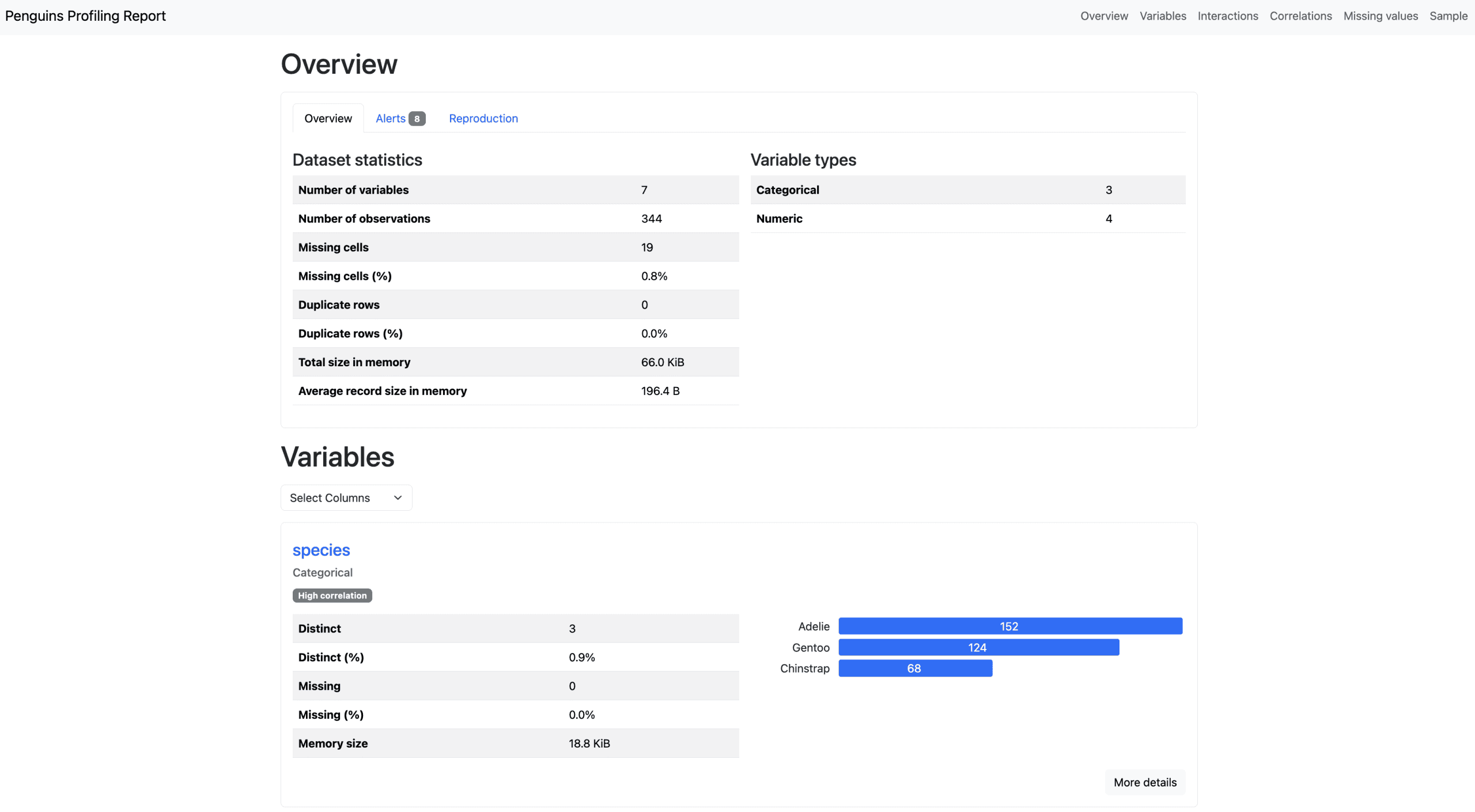
A piece of the generated profiling report
The one tradeoff is pace: a full report computes quite a bit, and it slows down on giant datasets. Two arguments repair that. Use minimal=True to change off the costliest computations, and profile a pattern fairly than the entire body if you simply want a really feel for the information:
profile = ProfileReport(df.pattern(frac=0.5), minimal=True)
There’s additionally a .evaluate() methodology for placing two datasets facet by facet — invaluable for recognizing drift between a coaching set and manufacturing knowledge, or between two time intervals.
# 6. Constructing a Actual “Desk 1” with tableone
Every part to date is for you — exploration aids. tableone is to your readers. It produces the stratified baseline-characteristics desk that opens practically each scientific and quantitative analysis paper (therefore “Desk 1”), with the formatting and statistics that reviewers count on.
from tableone import TableOne

knowledge = df.dropna(subset=["sex"])

columns     = ["bill_length_mm", "bill_depth_mm",
               "flipper_length_mm", "body_mass_g", "island", "sex"]
categorical = ["island", "sex"]
nonnormal   = ["body_mass_g"]   # summarize with median [IQR] as a substitute of imply (SD)

table1 = TableOne(
    knowledge,
    columns=columns,
    categorical=categorical,
    nonnormal=nonnormal,
    groupby="species",
    pval=True,
    smd=True,
)
print(table1.tabulate(tablefmt="github"))
The result’s a correctly formatted desk: steady variables as imply (SD), categoricals as n (%), something you flagged as non-normal as median [Q1,Q3] — stratified throughout your grouping variable, with a missing-data column, p-values, and standardized imply variations (SMD) between teams:
|                              |           | Lacking   | General                | Adelie                 | Chinstrap              | Gentoo                 | SMD (Adelie,Chinstrap)   | SMD (Adelie,Gentoo)   | SMD (Chinstrap,Gentoo)   | P-Worth   |
|------------------------------|-----------|-----------|------------------------|------------------------|------------------------|------------------------|--------------------------|-----------------------|--------------------------|-----------|
| n                            |           |           | 333                    | 146                    | 68                     | 119                    |                          |                       |                          |           |
| bill_length_mm, imply (SD)    |           | 0         | 44.0 (5.5)             | 38.8 (2.7)             | 48.8 (3.3)             | 47.6 (3.1)             | 3.315                    | 3.023                 | -0.393                   | <0.001    |
| bill_depth_mm, imply (SD)     |           | 0         | 17.2 (2.0)             | 18.3 (1.2)             | 18.4 (1.1)             | 15.0 (1.0)             | 0.062                    | -3.022                | -3.220                   | <0.001    |
| flipper_length_mm, imply (SD) |           | 0         | 201.0 (14.0)           | 190.1 (6.5)            | 195.8 (7.1)            | 217.2 (6.6)            | 0.837                    | 4.140                 | 3.119                    | <0.001    |
| body_mass_g, median [Q1,Q3]  |           | 0         | 4050.0 [3550.0,4775.0] | 3700.0 [3362.5,4000.0] | 3700.0 [3487.5,3950.0] | 5050.0 [4700.0,5500.0] | 0.064                    | 2.885                 | 3.043                    | <0.001    |
| island, n (%)                | Biscoe    |           | 163 (48.9)             | 44 (30.1)              | 0 (0.0)                | 119 (100.0)            | 1.819                    | 2.153                 | nan                      | <0.001    |
|                              | Dream     |           | 123 (36.9)             | 55 (37.7)              | 68 (100.0)             | 0 (0.0)                |                          |                       |                          |           |
|                              | Torgersen |           | 47 (14.1)              | 47 (32.2)              | 0 (0.0)                | 0 (0.0)                |                          |                       |                          |           |
| intercourse, n (%)                   | Feminine    |           | 165 (49.5)             | 73 (50.0)              | 34 (50.0)              | 58 (48.7)              | <0.001                   | 0.025                 | 0.025                    | 0.976     |
|                              | Male      |           | 168 (50.5)             | 73 (50.0)              | 34 (50.0)              | 61 (51.3)              |                          |                       |                          |           |
The actual payoff is export. A TableOne object goes straight to the format your manuscript wants — LaTeX (paste it into Overleaf), HTML, Markdown, or CSV:
table1.to_latex("table1.tex")
table1.to_html("table1.html")
table1.to_csv("table1.csv")
One vital factor that the bundle authors stress, and so will I: automated statistics will not be an alternative to judgment. The selection of which take a look at to run, whether or not a variable is actually regular, and find out how to deal with missingness all warrant human overview earlier than something goes to publication. tableone removes the tedium, not the duty.
# 7. Sprucing It right into a Publication-High quality Desk with Nice Tables
tableone codecs analysis tables particularly. For every other abstract — a enterprise report, a slide, or a README — Nice Tables turns a plain DataFrame right into a styled, presentation-ready desk, the identical approach the gt bundle does in R. It takes a Pandas or Polars body and renders to HTML or to a picture.
Take the customized abstract we constructed again in Step 3 and gown it up:
from great_tables import GT, md

numeric = df.select_dtypes("quantity")
stats = (numeric.agg(["mean", "median", "std", "min", "max"]).T
                .rename_axis("measurement").reset_index())
stats["missing_pct"] = df[numeric.columns].isna().imply().mul(100).values

desk = (
    GT(stats, rowname_col="measurement")
    .tab_header(title="Penguin Physique Measurements",
                subtitle="Descriptive statistics, Palmer Archipelago")
    .fmt_number(columns=["mean", "median", "std", "min", "max"], decimals=1)
    .fmt_percent(columns="missing_pct", decimals=1, scale_values=False)
    .data_color(columns="std", palette="Blues")
    .tab_source_note(md("Supply: *palmerpenguins* dataset (Horst et al.)."))
)
A number of issues are taking place right here. fmt_number and fmt_percent deal with show formatting so that you by no means hand-round once more. data_color applies a coloration gradient to the std column, drawing the attention to essentially the most variable measurements. tab_header and tab_source_note add the title and attribution that make a desk look completed. There’s lots extra — column spanners, conditional styling, even inline sparklines — however even this a lot produces one thing you’d fortunately put in entrance of stakeholders.
To make use of the consequence, render to an HTML string (works anyplace, no additional dependencies):
html = desk.as_raw_html()
with open("summary_table.html", "w") as f:
    f.write(html)
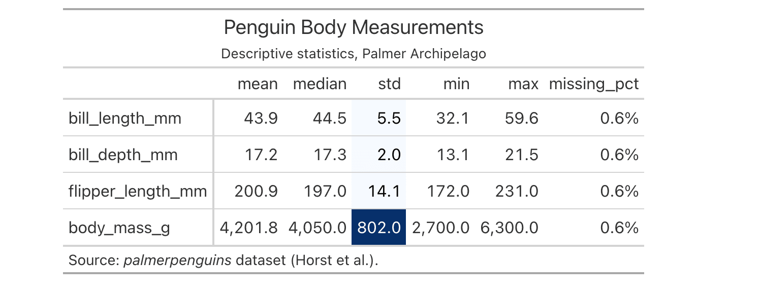
The styled Nice Tables output
# Tying It Collectively: One Perform, Each Time
The entire level of automation is repeatability. Wrap the pipeline so the following dataset is a single name:
from great_tables import GT, md

def descriptive_report(df, decimals=1):
    numeric = df.select_dtypes("quantity")
    stats = (numeric.agg(["count", "mean", "median", "std", "min", "max"]).T
                    .rename_axis("variable").reset_index())
    stats["missing_%"] = df[numeric.columns].isna().imply().mul(100).values
    return (
        GT(stats, rowname_col="variable")
        .tab_header(title="Descriptive Statistics",
                    subtitle=f"{len(df):,} rows x {df.form[1]} columns")
        .fmt_integer(columns="rely")
        .fmt_number(columns=["mean", "median", "std", "min", "max"], decimals=decimals)
        .fmt_percent(columns="missing_%", decimals=1, scale_values=False)
        .data_color(columns="std", palette="Blues")
        .tab_source_note(md("Generated routinely with pandas + Nice Tables."))
    )

descriptive_report(df)   # level it at any DataFrame
That is the distinction between a snippet and a instrument: you write it as soon as and reuse it on each dataset that lands in your desk.
# Wrapping Up
Descriptive statistics do not need to be a chore you re-implement on each mission. The ladder we climbed has a rung for each state of affairs:
- Pandas
describe()and.agg(): Zero dependencies, excellent for fast checks and customized summaries. - skimpy: A richer console abstract with histograms and missing-data percentages, in a single name.
- fg-data-profiling: An entire interactive HTML report if you want the total exploratory knowledge evaluation (EDA) image.
- tableone: The stratified “Desk 1” with p-values and SMDs for analysis papers, with one-line export to LaTeX, HTML, and CSV.
- Nice Tables: Polished, publication-quality styling for any abstract you’ve got produced.
Decide the lightest instrument that solutions your query. For a five-second sanity test, describe() wins. For a manuscript, tableone and Nice Tables earn their hold. And when you wrap your favourite mixture in a operate, you cease doing descriptive statistics and begin operating them — which is strictly the place you need to be so you possibly can spend your time on the evaluation that truly requires your mind.
Kanwal Mehreen is a machine studying engineer and a technical author with a profound ardour for knowledge science and the intersection of AI with drugs. She co-authored the e-book “Maximizing Productiveness with ChatGPT”. As a Google Era Scholar 2022 for APAC, she champions variety and tutorial excellence. She’s additionally acknowledged as a Teradata Range in Tech Scholar, Mitacs Globalink Analysis Scholar, and Harvard WeCode Scholar. Kanwal is an ardent advocate for change, having based FEMCodes to empower ladies in STEM fields.

