

Truncation and censoring are two distinct phenomena that trigger our samples to be incomplete. These phenomena come up in medical sciences, engineering, social sciences, and different analysis fields. If we ignore truncation or censoring when analyzing our knowledge, our estimates of inhabitants parameters might be inconsistent.
Truncation or censoring occurs through the sampling course of. Let’s start by defining left-truncation and left-censoring:
Our knowledge are left-truncated when people beneath a threshold should not current within the pattern. For instance, if we wish to research the dimensions of sure fish based mostly on the specimens captured with a web, fish smaller than the online grid gained’t be current in our pattern.
Our knowledge are left-censored at (kappa) if each particular person with a worth beneath (kappa) is current within the pattern, however the precise worth is unknown. This occurs, for instance, when now we have a measuring instrument that can’t detect values beneath a sure degree.
We are going to focus our dialogue on left-truncation and left-censoring, however the ideas we’ll talk about generalize to all forms of censoring and truncation—proper, left, and interval.
When performing estimations with truncated or censored knowledge, we have to use instruments that account for that sort of incomplete knowledge. For truncated linear regression, we are able to use the truncreg command, and for censored linear regression, we are able to use the intreg or tobit command.
On this weblog put up, we’ll analyze the traits of truncated and censored knowledge and talk about utilizing truncreg and tobit to account for the unfinished knowledge.
Truncated knowledge
Instance: Royal Marines
Fogel et al. (1978) revealed a dataset on the peak of Royal Marines that extends over two centuries. It may be used to find out the imply peak of males in Britain for various intervals of time. Trussell and Bloom (1979) level out that the pattern is truncated resulting from minimal peak restrictions for the recruits. The information are truncated (versus censored) as a result of people with heights beneath the minimal allowed peak don’t seem within the pattern in any respect. To account for this reality, they match a truncated distribution to the heights of Royal Marines from the interval 1800–1809.
We’re utilizing a man-made dataset based mostly on the issue described by Trussell and Bloom. We’ll assume that the inhabitants knowledge observe a traditional distribution with (mu=65) and (sigma=3.5), and that they’re left-truncated at 64.
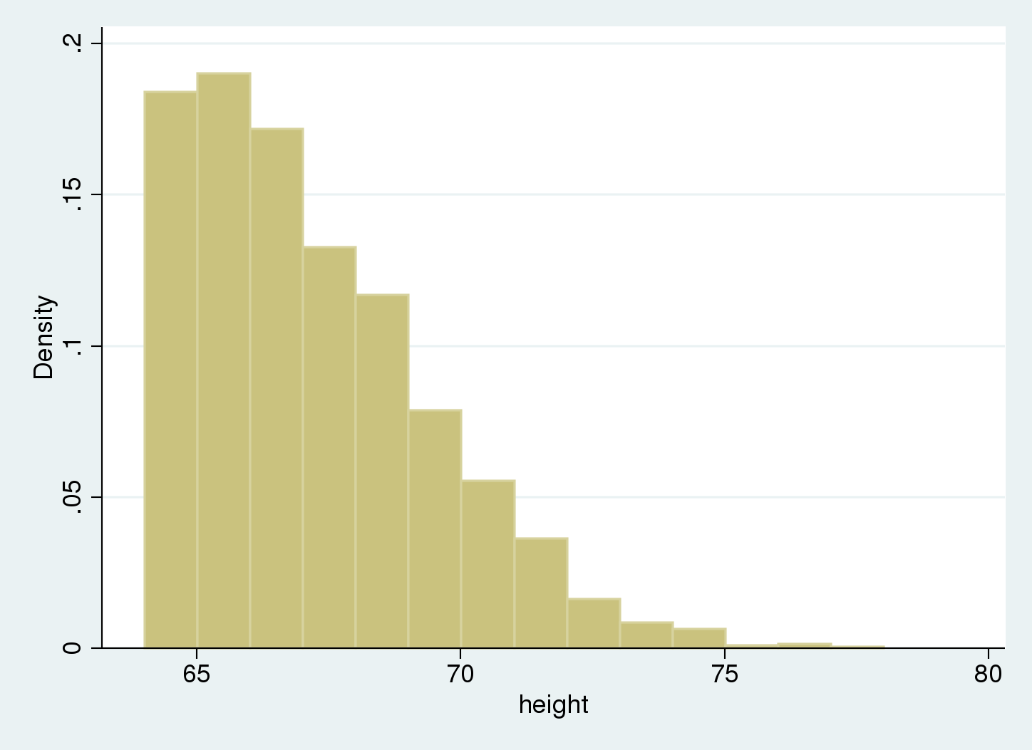
We use a histogram to summarize our knowledge.
We see there are not any knowledge beneath 64, our truncation level.
What occurs if we ignore truncation?
If we ignore the truncation and deal with the unfinished knowledge as full, the pattern common is inconsistent for the inhabitants imply, as a result of all observations beneath the truncation level are lacking. In our instance, the true imply is exterior the 95% confidence interval for
the estimated imply.
. imply peak

Imply estimation                   Variety of obs   =      2,200

--------------------------------------------------------------
             |       Imply   Std. Err.     [95% Conf. Interval]
-------------+------------------------------------------------
      peak |   67.18388   .0489487      67.08788    67.27987
--------------------------------------------------------------

. estat sd

-------------------------------------
             |       Imply   Std. Dev.
-------------+-----------------------
      peak |   67.18388    2.295898
-------------------------------------
We are able to examine the histogram of our pattern to the traditional distribution that we get if we ignore truncation, and take into account these values as estimates of the imply and normal deviation of the inhabitants.
. histogram peak , width(1)
>         addplot( operate f1 = normalden(x, 67.18, 2.30), vary(55 75))
(bin=14, begin=64.017105, width=1)
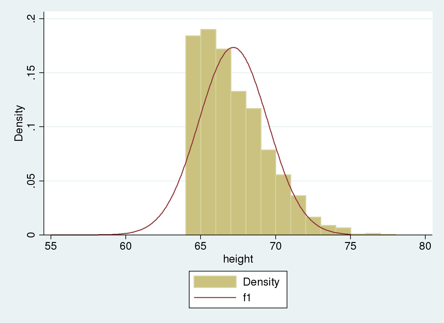
We see that the Gaussian density estimate, (f_1), which ignored truncation, is shifted to the correct of the histogram, and the variance appears to be underestimated. We are able to confirm this as a result of we used synthetic knowledge that have been simulated with an underlying imply of 65 and normal deviation of three.5 for the nontruncated distribution, versus the estimated imply of 67.2 and normal deviation of two.3.
Utilizing truncreg to account for truncation
We are able to use truncreg to estimate the parameters for the underlying nontruncated distribution; to account for the left-truncation at 64, we use choice ll(64).
. truncreg peak, ll(64)
(notice: 0 obs. truncated)

Becoming full mannequin:

Iteration 0:   log chance = -4759.5965
Iteration 1:   log chance =  -4603.043
Iteration 2:   log chance = -4600.5217
Iteration 3:   log chance = -4600.4862
Iteration 4:   log chance = -4600.4862

Truncated regression
Restrict:   decrease =         64                     Variety of obs     =      2,200
         higher =       +inf                     Wald chi2(0)      =          .
Log chance = -4600.4862                     Prob > chi2       =          .

------------------------------------------------------------------------------
      peak |      Coef.   Std. Err.      z    P>|z|     [95% Conf. Interval]
-------------+----------------------------------------------------------------
       _cons |   64.97701   .2656511   244.60   0.000     64.45634    65.49768
-------------+----------------------------------------------------------------
      /sigma |   3.506442   .1303335    26.90   0.000     3.250993    3.761891
------------------------------------------------------------------------------
Now, estimates are near our precise simulated values, (mu = 65), (sigma=3.5).
Let’s overlap the truncated density to the information histogram.
. histogram peak , width(1)
>   addplot(operate f_trunc =
>   cond(x<64, 0, normalden(x, 64.97, 3.51)/(1-normal((64-64.97)/3.51))),
>   vary(55 75))
(bin=14, begin=64.017105, width=1)
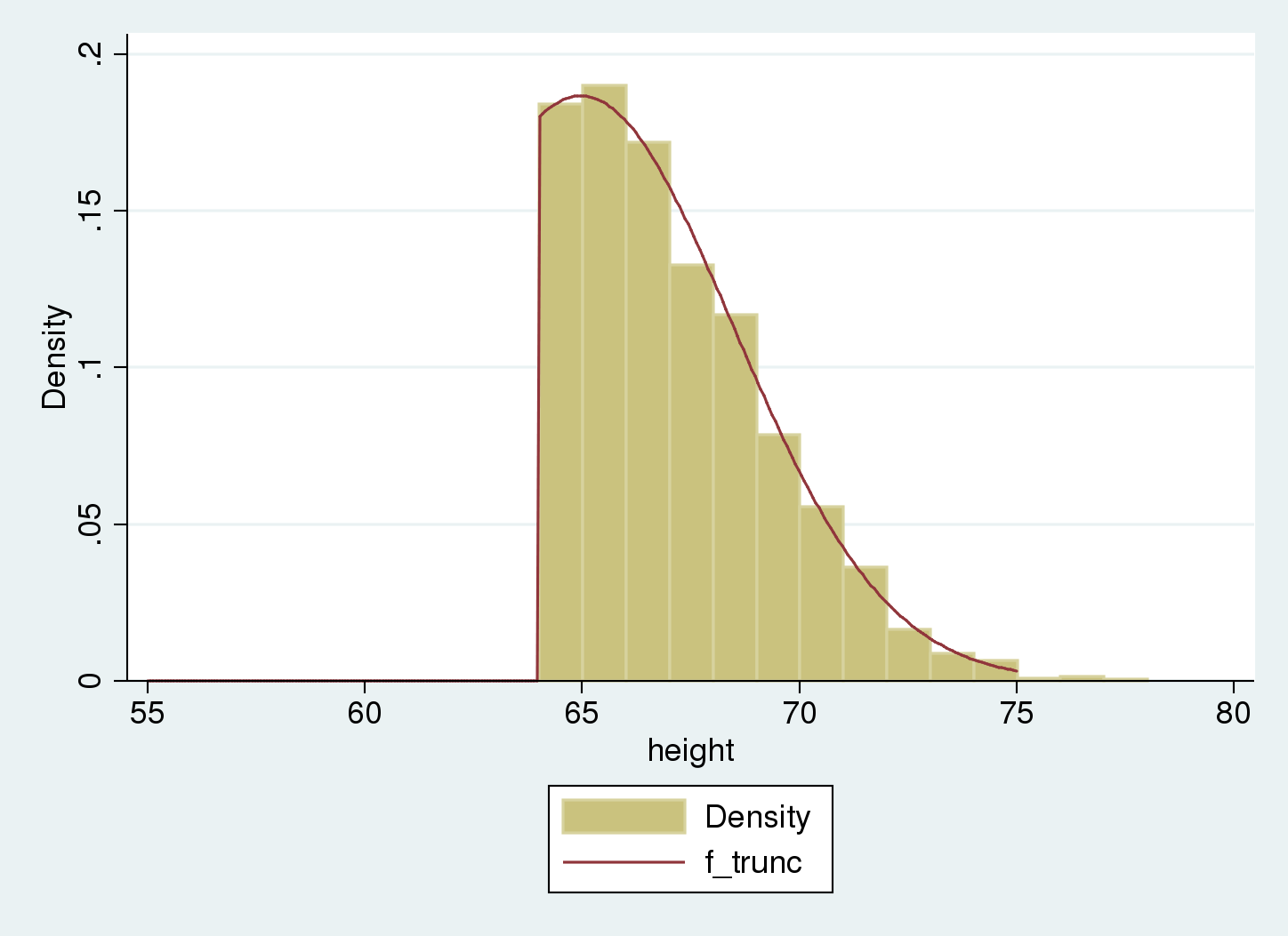
The truncated distribution matches our pattern. We estimate the inhabitants distribution as regular with imply equal to 65 and normal deviation equal to three.5.
Censored knowledge
Now we take into account an instance with censored knowledge slightly than truncated knowledge to display the distinction between the 2.
Instance: Nicotine ranges on family surfaces
Matt et al. (2004) carried out a research to evaluate contamination with tobacco smoke on surfaces in households of people who smoke. One measurement of curiosity was the extent of nicotine on furnishings surfaces. For every family, space wipe samples have been taken from the furnishings. Nonetheless, the measurement instrument couldn’t detect nicotine contamination beneath a sure restrict.
The information have been censored versus truncated. When the nicotine degree fell beneath the detection restrict, the remark was nonetheless included within the pattern with the nicotine degree recorded as being equal to that restrict.
I’ve created a man-made dataset loosely impressed by the issue on this research. The log of nicotine contamination ranges are assumed to be regular. Right here, lognlevel incorporates log nicotine ranges. The parameters used for simulating the log nicotine ranges for uncensored knowledge are (mu=ln(5)) and (sigma=2.5), and the information have been left-censored at 0.1. We begin by drawing a histogram.
. histogram lognlevel, width(.25)
(bin=53, begin=-2.3025851, width=.25)
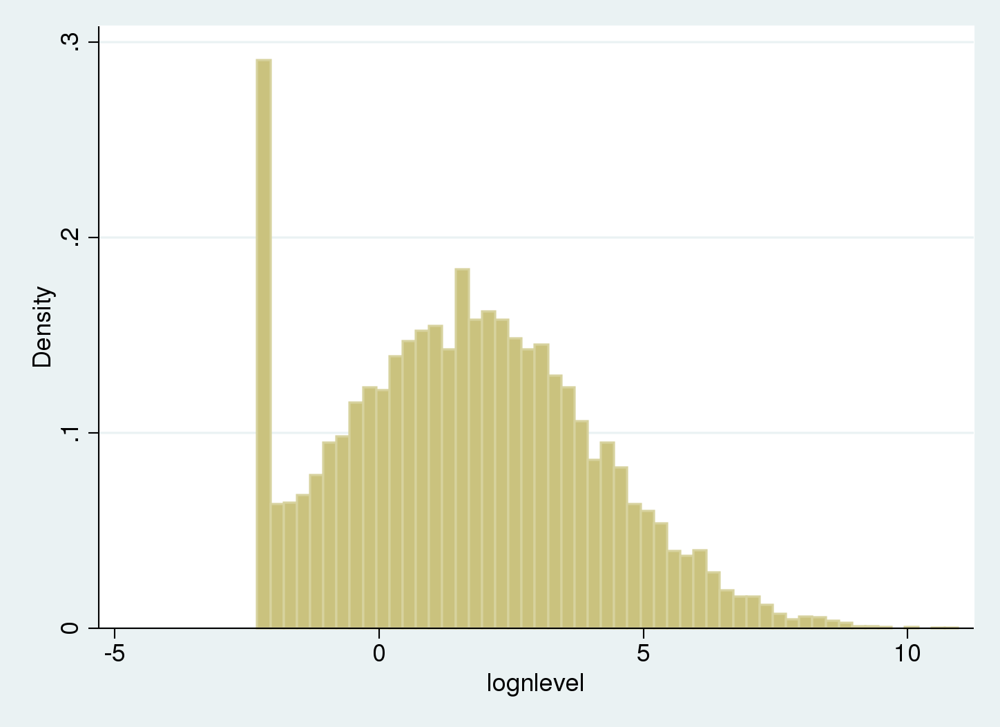
There’s a spike on the left of the histogram as a result of values beneath the restrict of detection (LOD) are recorded as being equal to the LOD.
Computing the uncooked imply and normal deviation for the pattern won’t present acceptable estimates for the underlying uncensored Gaussian distribution.
. summarize lognlevel

    Variable |        Obs        Imply    Std. Dev.       Min        Max
-------------+---------------------------------------------------------
   lognlevel |     10,000    1.683339    2.360516  -2.302585   10.73322
Imply and normal deviation are estimated as 1.68 and a pair of.4 respectively, the place the precise parameters are ln(5) =1.61 and a pair of.5.
Utilizing tobit to account for censoring
We estimate the imply and normal deviation of the distribution and account for the left-censoring through the use of tobit with the ll choice. (If censoring limits various amongst observations, we might use intreg as an alternative).
. tobit lognlevel, ll

Tobit regression                                Variety of obs     =     10,000
                                                LR chi2(0)        =       0.00
                                                Prob > chi2       =          .
Log chance = -22680.512                     Pseudo R2         =     0.0000

------------------------------------------------------------------------------
   lognlevel |      Coef.   Std. Err.      t    P>|t|     [95% Conf. Interval]
-------------+----------------------------------------------------------------
       _cons |   1.620857   .0249836    64.88   0.000     1.571884     1.66983
-------------+----------------------------------------------------------------
      /sigma |   2.486796   .0184318                      2.450666    2.522926
------------------------------------------------------------------------------
           588  left-censored observations at lognlevel <= -2.3025851
         9,412     uncensored observations
             0 right-censored observations
The underlying uncensored distribution is estimated as regular with imply 1.62 and normal deviation 2.49.
Let’s overlap the uncensored distribution to the histogram:
. histogram lognlevel , width(.25)
>  addplot( operate f = normalden(x, 1.62, 2.49), vary(-5 10))
(bin=53, begin=-2.3025851, width=.25)
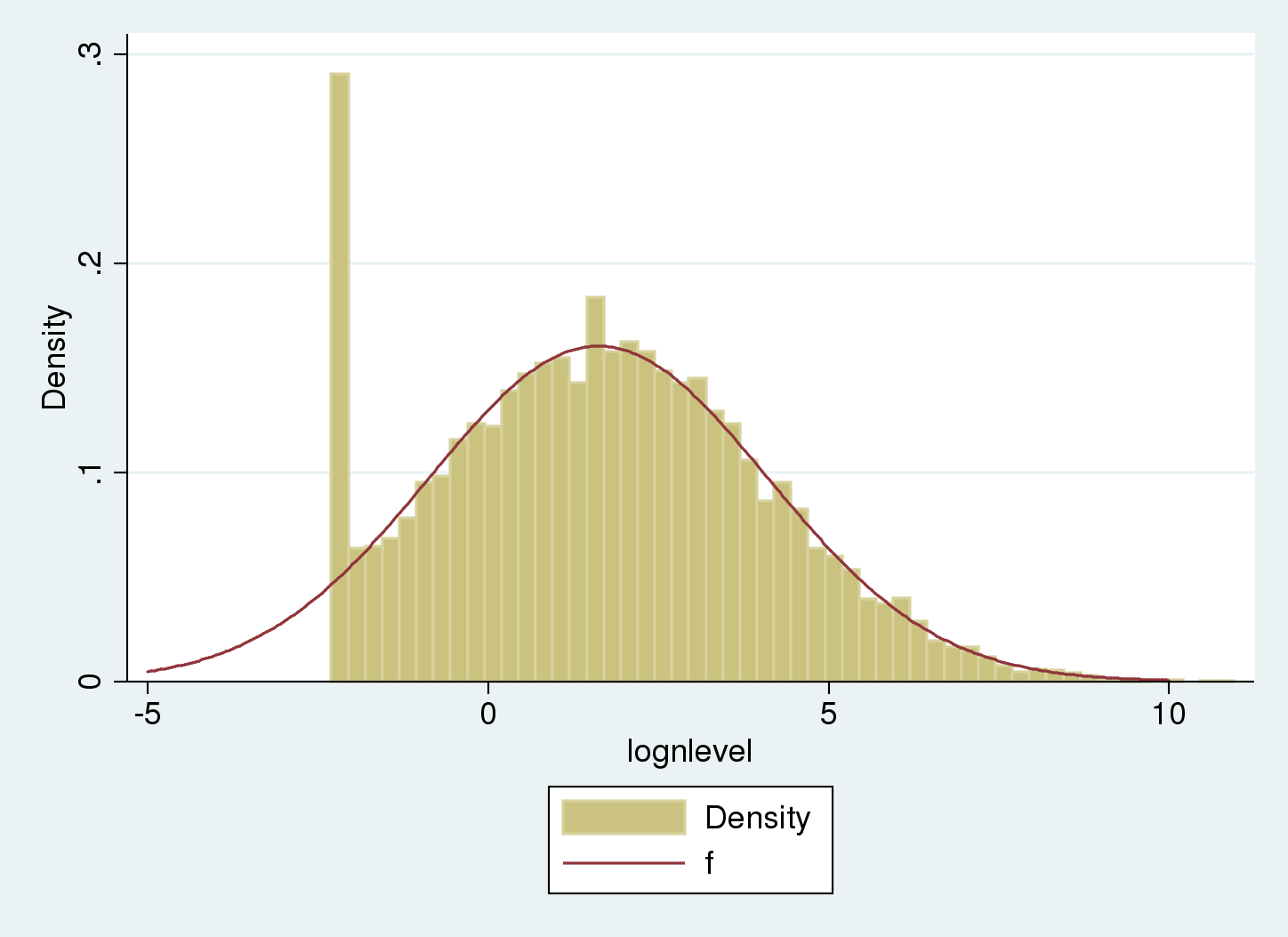
The underlying uncensored distribution matches the common a part of the histogram. The tail on the left compensates the spike on the censoring level.
Abstract
Censoring and truncation are two distinct phenomena that occur when sampling knowledge.
The underlying inhabitants parameters for a truncated Gaussian pattern will be estimated with truncreg. The underlying inhabitants parameters for a censored Gaussian pattern will be estimated with intreg or tobit.
Last remarks
We have mentioned the ideas of censoring and truncation, and proven examples for example these ideas.
There are some related factors associated to this dialogue that I wish to level out:
The dialogue above is predicated on the Gaussian mannequin, however the principle ideas prolong to any distribution.
The examples above match regression fashions with out covariates, so we are able to higher visualize the form of the censored and truncated distributions. Nonetheless, these ideas are simply prolonged to a regression framework with covariates the place the anticipated worth of a specific remark is a operate of the covariates.
I’ve mentioned using truncreg and tobit for censored and truncated knowledge. Nonetheless, these instructions may also be utilized to knowledge that aren’t truncated or censored however which might be sampled from a inhabitants with sure particular distributions.
References
Fogel, R. W., S. L. Engerman, J. Trussell, R. Floud, C. L. Pope and L. T. Wimmer. 1978.
The economics of mortality in North America, 1650–1910: An outline of a analysis challenge. Historic Strategies 11: 75–108.
Matt, G. E., P. J. E. Quintana, M. F. Hovell, J. T. Bernert, S. Track, N. Novianti, T. Juarez, J. Floro, C. Gehrman, M. Garcia, S. Larson. 2004. Households contaminated by environmental tobacco smoke: sources of toddler exposures. Tobacco Management 13: 27–29.
Trussell, J. and D. E. Bloom. 1979. A mannequin distribution of peak or weight at a given age. Human Biology 51: 523–536.