
")
The Abadie and Imbens (2011) bias correction for nearest neighbor matching will be written two methods. The usual presentation is imputation: you are expecting counterfactual outcomes at two factors, take the distinction, and subtract it out of your naive estimate. You’ll be able to consider their bias correction as utilizing regressions off the management group solely to then estimate a bias time period for the therapy and the management group utilizing these regression coefficients — a step which is legitimate below (and implied by) unconfoundedness as long as you’re keen to imagine a specific regression equation representing the end result modeling of Y(0) and its relationship to the covariates.
For individuals who are persevering with to deepen their information of regression adjustment, double sturdy estimators, and the Callaway and Sant’Anna estimator, which includes the Heckman, Ichimura and Todd (1997) regression adjustment technique, I feel a few of this previous Abadie and Imbens (2011) bias correction is unusually acquainted.
However I feel what I used to be nonetheless probably not anticipating is that that imputation technique off a regression may also be written down at the very same time another way as an augmentation, not simply an imputation. It’s an augmentation of the matched comparisons. You’re taking your matched management’s final result and regulate it straight by sliding alongside the regression line to account for the matching discrepancy. It’s the identical math, it’s the identical numbers, however perhaps only a totally different mind-set about the identical factor you’re doing? Possibly it’s a duality factor. Or perhaps it’s simply apparent to anybody who is aware of what a regression is doing.
Nonetheless, I discover the augmentation strategy fascinating as a result of it’s precisely how Ben-Michael et al. (2021) current their bias correction in augmented artificial management—and so they explicitly cite Abadie-Imbens because the inspiration. I knew they did that, and I even observed they’d transfer between two representations much like what I’m going to do. However for some purpose, I simply didn’t see it too on the similar time. And I’d by no means seen anybody present the equivalence cleanly for the cross-sectional matching case anyway. In order that’s what this put up does. I don’t suppose it deserves greater than a weblog put up, so I made a decision ultimately to place it right here.
Nearest neighbor matching has an issue: actual matches are uncommon with steady covariates. For those who match Andy (age 23) to Gina (age 26), and age impacts outcomes, you’ve launched bias as a result of unconfoundedness solely implies equal matches on common for teams with an identical covariate values. Technically, matching somebody 23 to 26 is a violation of that as you possibly can match 23 to 23 below unconfoundedness, however not 23 to 26. And it’s occurring since you’re working with a finite pattern, and typically you simply don’t have the matches there — an issue that will get worse, too, as the size you need to match on grows.
So, Abadie & Imbens (2011) confirmed this bias doesn’t vanish at √N price—the estimator isn’t √N-consistent with out correction. And subsequently their answer was to make use of regression to estimate and take away the bias from inexact matching.
Let me stroll you thru it step-by-step with the toy instance. Think about I’ve just a few folks within the knowledge like this. I wish to estimate the common therapy impact on the handled group (ATT) which implies discovering matches for Andy to Doug utilizing the untreated management group models Edith and onward. Assume too that Y(0) is unbiased of therapy project for teams of staff with the identical age (i.e., unconfoundedness or choice on observables). So then we do the match utilizing nearest neighbor matching which finds the set of matches that minimizes the sum of squared matching discrepancies.
However, if that sum of squared matching discrepancies is not zero, it means there may be probably some bias prompted, not by the fallacious covariates, however reasonably by having the fallacious matches. You have got approximate matches, not an identical ones, and to the diploma that related to every personnel for some covariates they’ve totally different common Y(0) values, then the therapy results are off by an quantity equal to the distinction between the handled unit’s Y(0) and the matched unit’s Y(0). Abadie and Imbens write that matching bias equation down and use it to then, below unconfoundedness, construct a regression-based bias correction technique which works like this:
-
Step 1: Match. Discover nearest neighbors. Andy → Gina/Hank (age 26). Naive ATT = $36.25, which is means off in my instance.
-
Step 2: Regress Y on X utilizing matched controls solely. That is the important thing element that may confuse folks—you don’t use all controls, simply those that have been really matched.
-
Step 3: Predict μ̂⁰(Xᵢ) and μ̂⁰(X_{j(i)}) for every handled unit and its match.
-
Step 4: Bias right.
(hat{delta}_i^{BC} = (Y_i – Y_{j(i)}) – (hat{mu}^0(X_i) – hat{mu}^0(X_{j(i)})))
In my case, the result’s an ATT of $4.167, which was right.
Let me present you this utilizing code, as I feel code usually makes issues much less summary. The canned process in Stata is teffects. In R, it’s matched (not matchit however reasonably matched). However I’ll present the teffects right here.
teffects nnmatch (earnings age) (d), atet biasadj(age)
Principally, you match as norma, however then after the comma you set biasdj(X). And what it does is run by these a number of steps I mentioned and regulate every unit’s particular person therapy results by an quantity equal to the hole of their imputed Y(0) outcomes.
Right here’s the way you do it manually, not utilizing canned software program.
* Match and get match IDs
teffects nnmatch (earnings age) (d), atet gen(match)

* Establish matched controls
* Regress Y on X utilizing ONLY matched controls
reg earnings age if matched_control == 1

* Predict at handled X and match's X
predict muhat0

* Bias right: subtract the distinction
gen te_bc = te - (muhat_treated - muhat_match)
In my instance, within the new e book, I present that this additionally offers you an ATT of 4.167.
On the finish of this substack, I inform how I solely discovered this whereas writing the e book as a result of I received caught being unable to maneuver between what teffects was doing above to a guide technique (additionally above), it doesn’t matter what I did. I stored shrinking the dataset to being the smallest measurement potential in order that I might determine simply the place my mistake was coming in, which led me to understand it should be I had a flaw in my understanding. Because it seems, as I say on the finish, I by no means realized that I needed to do the imputation off the matched pattern solely as a result of I used to be misunderstanding some subtleties from the Abadie and Imbens (2011) notation. You need to actually be listening to see it, too, which I clarify on the finish.
But it surely was type of serendipitous in a means as a result of since I couldn’t get it proper, I went on this wild goose chase making an attempt to get the guide correction to work for the sake of the e book, purely as an illustration, and I ended up on the fallacious spot that I’m calling “augmentation” as a result of, like I mentioned, it’s fairly much like Ben-Michael, Feller, and Rothstein’s (2021) augmented artificial management paper—which explicitly cites Abadie-Imbens as their inspiration.
For individuals who know OLS inside-out, the equivalence might be apparent. However not everybody sees it instantly, and typically a distinct angle reveals one thing helpful. Principally the augmentation instinct is to as a substitute of predicting at two factors and subtracting, take the match’s precise final result and slide it alongside the regression line to the place the handled unit sits like this:
(hat{Y}^0_{aug,i} = Y_{j(i)} + hat{beta}(X_i – X_{j(i)}))
Discover what you’re doing. You’ve received a matched management group unit, j(i). She’s been matched to your handled unit i in different phrases which is why I write it down as j(i). She’s the jth unit matched to the ith unit — therefore j(i). Within the Abadie and Imbens (2011), there was a delicate transfer the place the notation went again to utilizing j, because it referenced an earlier equation that had made that clearer I feel, and I simply couldn’t see the forest for the timber so stored working the regressions off your complete pattern, not the matched pattern. Anyway, apparent now nevertheless it wasn’t apparent then to me in any respect.
Let me present the variations to you now of them facet by facet.
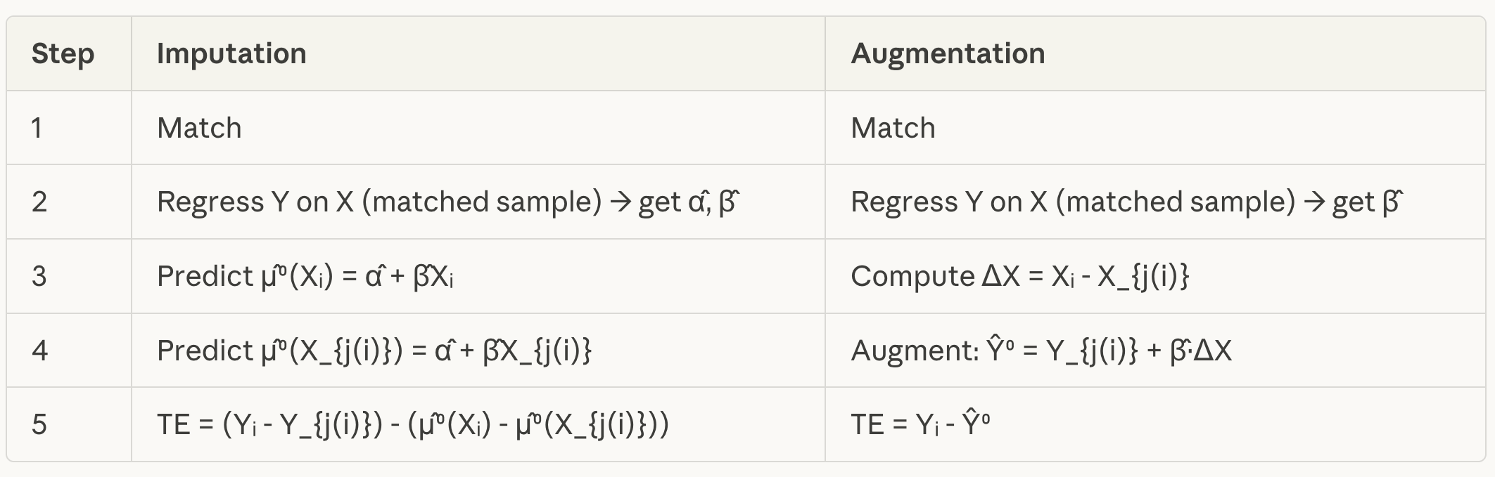
Discover that on the imputation facet, the bias correction is known as that since you’re subtracting the estimated bias in step 5 from the individually estimated therapy results. As soon as you’re taking the common over these TE values for the handled unit, you will have an ATT estimate, and simply should get a typical error.
On the suitable, you begin on the similar place — you do the closest neighbor matching. After which step 2 is identical as nicely — you regress Y onto X utilizing the matched management group pattern solely. On this sense, it’s straight up regression adjustment — regress Y onto X for management group solely (solely right here it’s the management group matched pattern solely). Then use these regression coefficients.
However look right here. Whereas in step 3 for imputation, you probably did imputation for the therapy group with these management group regression coefficients (after which in step 4, did it once more for the matched pattern management group), within the augmentation strategy, you calculate a brand new matching discreprancy which I referred to as Delta X. That Delta X is not in regards to the final result, discover. See that? See how step 3 is not in regards to the final result? Fairly, it’s the hole between every unit’s age (on this instance) and the matched unit’s age. For those who had good matches, then that will be zero, however should you had approximate matches, it might be non-zero. It’d be “optimum” from the angle of minimizing distance, however it might be technically the very best of the worst case conditions.
Step 4 then merely provides to every management group out the matching discreprancy multiplied by the slope coefficient. And that’s the new Y(0) for the j(i) unit. You then within the last step calculate the person therapy impact as nothing greater than this:
(TE_i = Y_i – widehat{Y}_i^0)
the place the second time period is solely the matched comparability group final result plus the slope coefficient multiplied by the matching discreprancy. And that’s numerically an identical to doing imputation steps within the first column. Right here’s the code.
* Step 1: Match
teffects nnmatch (earnings age) (d), atet gen(match)

* Step 2: Regress on matched controls, save coefficient
reg earnings age if matched_control == 1
native beta = _b[age]

* Step 3: Increase every matched final result
gen y0_augmented = y0_match + `beta' * (age_treated - age_match)

* Step 4: Remedy impact
gen te_bc = y1 - y0_augmented
After which should you do this in my e book instance, you get an ATT of 4.167 which is identical reply as teffects and is identical reply the imputation guide technique.
So what’s going on? Let me present you by beginning with the augmentation written out.
(hat{delta}_i^{BC} = Y_i – Y_{j(i)} – hat{beta}(X_i – X_{j(i)}))
If we rewrite our imputation bias right, we get this:
(hat{mu}^0(X_i) – hat{mu}^0(X_{j(i)}) = (hat{alpha} + hat{beta}X_i) – (hat{alpha} + hat{beta}X_{j(i)}) = hat{beta}(X_i – X_{j(i)}))
Discover that once I rewrote the differenced mu phrases from the imputation technique into their corresponding “proper hand facet” regression elements, the α̂ (the intercept) cancels out. We used the intercept to get imputed potential outcomes, however as a result of we differenced them, they then canceled out. That was really not apparent to me till I did this augmentation for some purpose. However you possibly can see it there in that line what occurs — the intercepts one, leaving solely the second time period of every expression, and once we group the phrases, we get the augmentation expression as slope occasions matching discreprancy. And so for the reason that first phrases and the final phrases are the identical, each of them modify the individually estimated therapy results within the an identical means, which is that this:
(hat{delta}_i^{BC} = (Y_i – Y_{j(i)}) – (hat{mu}^0(X_i) – hat{mu}^0(X_{j(i)})))
Which is the Abadie and Imbens (2011) imputation components, however which you may simply as simply written this manner:
(hat{delta}_i^{BC} = Y_i – Y_{j(i)} – widehat{beta}(X_i – X_{j(i)}))
That they’re in truth the identical factor.
So, what does this should do with artificial management? Nothing straight — not till a decade later anyway when Ben-Michael, Feller, and Rothstein (2021) wrote:
“Analogous to bias correction for inexact matching (Rubin, 1973; Abadie and Imbens, 2011), ASCM begins with the unique SCM estimate, makes use of an final result mannequin to estimate the bias because of imperfect pre-treatment match, after which makes use of this to de-bias the estimate.”
Right here is their augmentation of the unique Abadie artificial management. Their components is:
(hat{Y}^0_{aug} = sum_j w_j Y_j + hat{beta}’ left( X_1 – sum_j w_j X_j proper))
Which his the identical construction as what I simply confirmed you: begin with the match (i.e., the artificial management discovered utilizing Abadie’s technique), however then regulate it by (slope × covariate discrepancy). Which is identical factor I simply confirmed you, solely within the context of artificial management. Fascinating proper?
That’s the million greenback query, and it’s why I couldn’t determine what to do with this as soon as I labored it out. I assumed perhaps it may very well be a word or one thing, however I made a decision I didn’t actually know. So I simply opted to put in writing it right here. However the factor is, it’s potential perhaps that should you noticed this bias correction as an augmentation of an identical discrepancy off of a regression, maybe you is perhaps impressed to see some type of repair that’s in any other case opaque to you should you solely noticed it as an imputation?
I imply, imputation and augmentations aren’t precisely the identical factor — that’s what makes it bizarre to me that they transform the identical factor. Imputation is about outcomes for 2 teams; augmentation is about covariates for 2 teams. It’s simply that because you’re differencing the outcomes primarily based off a regression of the end result onto the covariates, then it does technically turn out to be the identical factor. And but, the variable Y and the variable X aren’t technically the identical column of numbers. Which is why I’m scripting this as if to say perhaps you possibly can see one thing should you’re targeted on X that you just in any other case couldn’t see should you have been targeted on Y?
As an example, take the Wald estimator in instrumental variables. That’s this:
(delta_{Wald} = fracZ=1] – E[YZ=0])
The numerator is the lowered type; the denominator is the primary stage. Properly, you possibly can present with only some steps that that equation is numerically an identical to 2 stage least squares, despite the fact that two stage least squares has an early step of utilizing a regression of D onto the instrument, Z, getting fitted values of D after which working a regression of the end result onto these fitted values.
I imply, that’s actually an identical to the Wald estimator with out covariates. And I feel lots of people — perhaps not you, however undoubtedly lots of people — don’t instantly see that that’s the case. It’s lots of steps frankly. It’s a presentation of concepts in uncommon methods utilizing regressions. I simply suppose for some, it’s apparent, and others it’s not apparent.
Properly, perhaps this equivalence between augmentation and imputation is identical factor. Possibly it’s extremely apparent to some — nearly boringly so — and to others it turns the lights on. Not simply to bias correction strategies, however perhaps even to delicate issues with regressions themselves. It’s about shifting from the suitable of the equal signal to the left of the equal signal. It’s about what occurs once you take variations and each phrases have a continuing. It’s little issues however all it takes is 2 or 3 little issues to maintain one thing from being apparent.
Whether or not that decomposition is beneficial for something past pedagogy? I genuinely don’t know. However I figured I’d write it up in case another person finds it useful—or sees one thing I missed.