The Wilson Confidence Interval for a Proportion

Suppose that we observe a random pattern (X_1, dots, X_n) from a traditional inhabitants with unknown imply (mu) and identified variance (sigma^2). Below these assumptions, the pattern imply (bar{X}_n equiv left(frac{1}{n} sum_{i=1}^n X_iright)) follows a (N(mu, sigma^2/n)) distribution. Centering and standardizing,
[ frac{bar{X}_n – mu}{sigma/sqrt{n}} sim N(0,1).]
Now, suppose we need to take a look at (H_0colon mu = mu_0) towards the two-sided different (H_1colon mu = mu_0) on the 5% significance stage. If (mu = mu_0), then the take a look at statistic
[T_n equiv frac{bar{X}_n – mu_0}{sigma/sqrt{n}}]
follows a normal regular distribution. If (mu neq mu_0), then (T_n) doesn’t comply with a normal regular distribution. To hold out the take a look at, we reject (H_0) if (|T_n|) is bigger than (1.96), the ((1 – alpha/2)) quantile of a normal regular distribution for (alpha = 0.05). To place it one other means, we fail to reject (H_0) if (|T_n| leq 1.96). So for what values of (mu_0) will we fail to reject? By the definition of absolute worth and the definition of (T_n) from above, (|T_n| leq 1.96) is equal to
[
– 1.96 leq frac{bar{X}_n – mu_0}{sigma/sqrt{n}} leq 1.96.
]
Re-arranging, this in flip is equal to
[
bar{X}_n – 1.96 times frac{sigma}{sqrt{n}} leq mu_0 leq bar{X}_n + 1.96 times frac{sigma}{sqrt{n}}.
]
This tells us that the values of (mu_0) we’ll fail to reject are exactly people who lie within the interval (bar{X} pm 1.96 occasions sigma/sqrt{n}). Does this look acquainted? It ought to: it’s the standard 95% confidence interval for a the imply of a traditional inhabitants with identified variance. The 95% confidence interval corresponds precisely to the set of values (mu_0) that we fail to reject on the 5% stage.

This instance is a particular case a extra normal consequence. In the event you give me a ((1 – alpha)occasions 100%) confidence interval for a parameter (theta), I can use it to check (H_0colon theta = theta_0) towards (H_0 colon theta neq theta_0). All I’ve to do is examine whether or not (theta_0) lies inside the boldness interval, through which case I fail to reject, or outdoors, through which case I reject. Conversely, in the event you give me a two-sided take a look at of (H_0colon theta = theta_0) with significance stage (alpha), I can use it to assemble a ((1 – alpha) occasions 100%) confidence interval for (theta). All I’ve to do is acquire the values of (theta_0) which are not rejected. This process known as inverting a take a look at.

Across the similar time as we train college students the duality between testing and confidence intervals–you need to use a confidence interval to hold out a take a look at or a take a look at to assemble a confidence interval–we throw a wrench into the works. Probably the most commonly-presented take a look at for a inhabitants proportion (p) does not coincide with probably the most commonly-presented confidence interval for (p). To cite from web page 355 of Kosuke Imai’s improbable textbook Quantitative Social Science: An Introduction

the usual error used for confidence intervals is completely different from the usual error used for speculation testing. It’s because the latter customary error is derived below the null speculation … whereas the usual error for confidence intervals is computed utilizing the estimated proportion.

Let’s translate this into arithmetic. Suppose that (X_1, …, X_n sim textual content{iid Bernoulli}(p)) and let (widehat{p} equiv (frac{1}{n} sum_{i=1}^n X_i)). The 2 customary errors that Imai describes are
[
text{SE}_0 equiv sqrt{frac{p_0(1 – p_0)}{n}} quad text{versus} quad
widehat{text{SE}} equiv sqrt{frac{widehat{p}(1 – widehat{p})}{n}}.
]
Following the recommendation of our introductory textbook, we take a look at (H_0colon p = p_0) towards (H_1colon p neq p_0) on the (5%) stage by checking whether or not (|(widehat{p} – p_0) / textual content{SE}_0|) exceeds (1.96). That is referred to as the rating take a look at for a proportion. Once more following the recommendation of our introductory textbook, we report (widehat{p} pm 1.96 occasions widehat{textual content{SE}}) as our 95% confidence interval for (p). As you could recall from my earlier publish, that is the so-called Wald confidence interval for (p). As a result of the 2 customary error formulation typically disagree, the connection between checks and confidence intervals breaks down.

To make this extra concrete, let’s plug in some numbers. Suppose that (n = 25) and our noticed pattern accommodates 5 ones and 20 zeros. Then (widehat{p} = 0.2) and we will calculate (widehat{textual content{SE}}) and the Wald confidence interval as follows

n <- 25
n1 <- 5
p_hat <- n1 / n
alpha <- 0.05
SE_hat <- sqrt(p_hat * (1 - p_hat) / n)
p_hat + c(-1, 1) * qnorm(1 - alpha / 2) * SE_hat

## [1] 0.04320288 0.35679712

The worth 0.07 is effectively inside this interval. This implies that we must always fail to reject (H_0colon p = 0.07) towards the two-sided different. However after we compute the rating take a look at statistic we acquire a worth effectively above 1.96, in order that (H_0colon p = 0.07) is soundly rejected:

p0 <- 0.07
SE0 <- sqrt(p0 * (1 - p0) / n)
abs((p_hat - p0) / SE0)

## [1] 2.547551

The take a look at says reject (H_0colon p = 0.07) and the boldness interval says don’t. Upon encountering this instance, your college students resolve that statistics is a tangled mess of contradictions, despair of ever making sense of it, and resign themselves to easily memorizing the requisite formulation for the examination.

How can we dig our means out of this mess? One thought is to use a special take a look at, one which agrees with the Wald confidence interval. If we had used (widehat{textual content{SE}}) reasonably than (textual content{SE}_0) to check (H_0colon p = 0.07) above, our take a look at statistic would have been

abs((p_hat - p0) / SE_hat)

## [1] 1.625

which is clearly lower than 1.96. Thus we might fail to reject (H_0colon p = 0.7) precisely because the Wald confidence interval instructed us above. This process known as the Wald take a look at for a proportion. Its essential profit is that it agrees with the Wald interval, in contrast to the rating take a look at, restoring the hyperlink between checks and confidence intervals that we train our college students. Sadly the Wald confidence interval is horrible and you must by no means use it. As a result of the Wald take a look at is equal to checking whether or not (p_0) lies contained in the Wald confidence interval, it inherits all the latter’s defects.

Certainly, in comparison with the rating take a look at, the Wald take a look at is a catastrophe, as I’ll now present. Suppose we feature out a 5% take a look at. If the null is true, we must always reject it 5% of the time. As a result of the Wald and Rating checks are each primarily based on an approximation supplied by the central restrict theorem, we must always permit a little bit of leeway right here: the precise rejection charges could also be barely completely different from 5%. However, we’d count on them to at the least be pretty shut to the nominal worth of 5%. The next plot reveals the precise kind I error charges of the rating and Wald checks, over a variety of values for the true inhabitants proportion (p) with pattern sizes of 25, 50, and 100. In every case the nominal dimension of every take a look at, proven as a dashed purple line, is 5%.

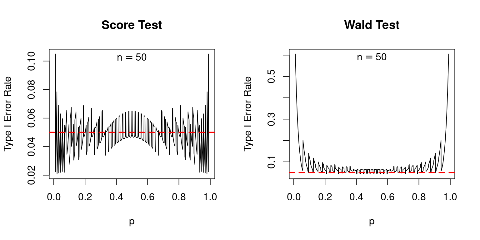
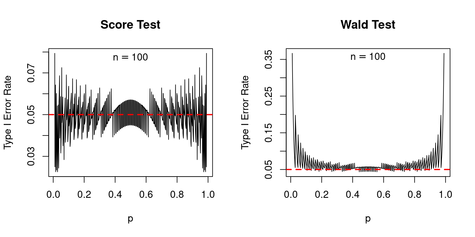
The rating take a look at isn’t excellent: if (p) is extraordinarily near zero or one, its precise kind I error charge could be appreciably greater than its nominal kind I error charge: as a lot as 10% in comparison with 5% when (n = 25). However typically, its efficiency is nice. In distinction, the Wald take a look at is completely horrible: its nominal kind I error charge is systematically greater than 5% even when (n) will not be particularly small and (p) will not be particularly near zero or one.

Granted, instructing the Wald take a look at alongside the Wald interval would cut back confusion in introductory statistics programs. However it could additionally equip college students with awful instruments for real-world inference. There’s a higher means: reasonably than instructing the take a look at that corresponds to the Wald interval, we might train the confidence interval that corresponds to the rating take a look at.

Suppose we acquire all values (p_0) that the rating take a look at does not reject on the 5% stage. If the rating take a look at is working effectively–if its nominal kind I error charge is shut to five%–the ensuing set of values (p_0) can be an approximate ((1 – alpha) occasions 100%) confidence interval for (p). Why is that this so? Suppose that (p_0) is the true inhabitants proportion. Then an interval constructed on this means will cowl (p_0) exactly when the rating take a look at doesn’t reject (H_0colon p = p_0). This happens with likelihood ((1 – alpha)). As a result of the rating take a look at is way more correct than the Wald take a look at, the boldness interval that we acquire by inverting it means can be way more correct than the Wald interval. This interval known as the rating interval or the Wilson interval.

So let’s do it: let’s invert the rating take a look at. Our purpose is to seek out all values (p_0) such that (|(widehat{p} – p_0)/textual content{SE}_0|leq c) the place (c) is the conventional essential worth for a two-sided take a look at with significance stage (alpha). Squaring each side of the inequality and substituting the definition of (textual content{SE}_0) from above offers
[
(widehat{p} – p_0)^2 leq c^2 left[ frac{p_0(1 – p_0)}{n}right].
]
Multiplying each side of the inequality by (n), increasing, and re-arranging leaves us with a quadratic inequality in (p_0), specifically
[
(n + c^2) p_0^2 – (2nwidehat{p} + c^2) p_0 + nwidehat{p}^2 leq 0.
]
Bear in mind: we’re looking for the values of (p_0) that fulfill the inequality. The phrases ((n + c^2)) together with ((2nwidehat{p})) and (nwidehat{p}^2) are constants. As soon as we select (alpha), the essential worth (c) is thought. As soon as we observe the info, (n) and (widehat{p}) are identified. Since ((n + c^2) > 0), the left-hand aspect of the inequality is a parabola in (p_0) that opens upwards. Because of this the values of (p_0) that fulfill the inequality should lie between the roots of the quadratic equation
[
(n + c^2) p_0^2 – (2nwidehat{p} + c^2) p_0 + nwidehat{p}^2 = 0.
]
By the quadratic components, these roots are
[
p_0 = frac{(2 nwidehat{p} + c^2) pm sqrt{4 c^2 n widehat{p}(1 – widehat{p}) + c^4}}{2(n + c^2)}.
]
Factoring (2n) out of the numerator and denominator of the right-hand aspect and simplifying, we will re-write this as
[
begin{align*}
p_0 &= frac{1}{2left(n + frac{n c^2}{n}right)}left{left(2nwidehat{p} + frac{2n c^2}{2n}right) pm sqrt{4 n^2c^2 left[frac{widehat{p}(1 – widehat{p})}{n}right] + 4n^2c^2left[frac{c^2}{4n^2}right] }proper}
p_0 &= frac{1}{2nleft(1 + frac{ c^2}{n}proper)}left{2nleft(widehat{p} + frac{c^2}{2n}proper) pm 2ncsqrt{ frac{widehat{p}(1 – widehat{p})}{n} + frac{c^2}{4n^2}} proper}

p_0 &= left( frac{n}{n + c^2}proper)left{left(widehat{p} + frac{c^2}{2n}proper) pm csqrt{ widehat{textual content{SE}}^2 + frac{c^2}{4n^2} }proper}
finish{align*}
]
utilizing our definition of (widehat{textual content{SE}}) from above. And there you will have it: the right-hand aspect of the ultimate equality is the ((1 – alpha)occasions 100%) Wilson confidence interval for a proportion, the place (c = texttt{qnorm}(1 – alpha/2)) is the conventional essential worth for a two-sided take a look at with significance stage (alpha), and (widehat{textual content{SE}}^2 = widehat{p}(1 – widehat{p})/n).

In comparison with the Wald interval, (widehat{p} pm c occasions widehat{textual content{SE}}), the Wilson interval is actually extra sophisticated. However it’s constructed from precisely the identical info: the pattern proportion (widehat{p}), two-sided essential worth (c) and pattern dimension (n). Computing it by hand is tedious, however programming it in R is a snap:

get_wilson_CI <- perform(x, alpha = 0.05) {
  #-----------------------------------------------------------------------------
  # Compute the Wilson (aka Rating) confidence interval for a popn. proportion
  #-----------------------------------------------------------------------------
  # x        vector of information (zeros and ones)
  # alpha    1 - (confidence stage)
  #-----------------------------------------------------------------------------
  n <- size(x)
  p_hat <- imply(x)
  SE_hat_sq <- p_hat * (1 - p_hat) / n
  crit <- qnorm(1 - alpha / 2)
  omega <- n / (n + crit^2)
  A <- p_hat + crit^2 / (2 * n)
  B <- crit * sqrt(SE_hat_sq + crit^2 / (4 * n^2))
  CI <- c('decrease' = omega * (A - B), 
          'higher' = omega * (A + B))
  return(CI)
}

Discover that that is solely barely extra sophisticated to implement than the Wald confidence interval:

get_wald_CI <- perform(x, alpha = 0.05) {
  #-----------------------------------------------------------------------------
  # Compute the Wald confidence interval for a popn. proportion
  #-----------------------------------------------------------------------------
  # x        vector of information (zeros and ones)
  # alpha    1 - (confidence stage)
  #-----------------------------------------------------------------------------
  n <- size(x)
  p_hat <- imply(x)
  SE_hat <- sqrt(p_hat * (1 - p_hat) / n)
  ME <- qnorm(1 - alpha / 2) * SE_hat
  CI <- c('decrease' = p_hat - ME, 
          'higher' = p_hat + ME)
  return(CI)
}

With a pc reasonably than pen and paper there’s little or no price utilizing the extra correct interval. Certainly, the built-in R perform prop.take a look at() reviews the Wilson confidence interval reasonably than the Wald interval:

set.seed(1234)
x <- rbinom(20, 1, 0.5)
prop.take a look at(sum(x), size(x), right = FALSE) # no continuity correction

## 
##  1-sample proportions take a look at with out continuity correction
## 
## knowledge:  sum(x) out of size(x), null likelihood 0.5
## X-squared = 0.2, df = 1, p-value = 0.6547
## different speculation: true p will not be equal to 0.5
## 95 % confidence interval:
##  0.3420853 0.7418021
## pattern estimates:
##    p 
## 0.55

get_wilson_CI(x)

##     decrease     higher 
## 0.3420853 0.7418021

You might cease studying right here and easily use the code from above to assemble the Wilson interval. However computing is barely half the battle: we need to perceive our measures of uncertainty. Whereas the Wilson interval could look considerably unusual, there’s really some quite simple instinct behind it. It quantities to a compromise between the pattern proportion (widehat{p}) and (1/2).

The Wald estimator is centered round (widehat{p}), however the Wilson interval will not be.
Manipulating our expression from the earlier part, we discover that the midpoint of the Wilson interval is
[
begin{align*}
widetilde{p} &equiv left(frac{n}{n + c^2} right)left(widehat{p} + frac{c^2}{2n}right) = frac{n widehat{p} + c^2/2}{n + c^2}
&= left( frac{n}{n + c^2}right)widehat{p} + left( frac{c^2}{n + c^2}right) frac{1}{2}
&= omega widehat{p} + (1 – omega) frac{1}{2}
end{align*}
]
the place the burden (omega equiv n / (n + c^2)) is at all times strictly between zero and one. In different phrases, the middle of the Wilson interval lies between (widehat{p}) and (1/2). In impact, (widetilde{p}) pulls us away from excessive values of (p) and in direction of the center of the vary of potential values for a inhabitants proportion. For a hard and fast confidence stage, the smaller the pattern dimension, the extra that we’re pulled in direction of (1/2). For a hard and fast pattern dimension, the upper the boldness stage, the extra that we’re pulled in direction of (1/2).

Persevering with to make use of the shorthand (omega equiv n /(n + c^2)) and (widetilde{p} equiv omega widehat{p} + (1 – omega)/2), we will write the Wilson interval as
[
widetilde{p} pm c times widetilde{text{SE}}, quad widetilde{text{SE}} equiv omega sqrt{widehat{text{SE}}^2 + frac{c^2}{4n^2}}.
]
So what can we are saying about (widetilde{textual content{SE}})? It seems that the worth (1/2) is lurking behind the scenes right here as effectively. The simplest strategy to see that is by squaring (widehat{textual content{SE}}) to acquire
[
begin{align*}
widetilde{text{SE}}^2 &= omega^2left(widehat{text{SE}}^2 + frac{c^2}{4n^2} right) = left(frac{n}{n + c^2}right)^2 left[frac{widehat{p}(1 – widehat{p})}{n} + frac{c^2}{4n^2}right]
&= frac{1}{n + c^2} left[frac{n}{n + c^2} cdot widehat{p}(1 – widehat{p}) + frac{c^2}{n + c^2}cdot frac{1}{4}right]
&= frac{1}{widetilde{n}} left[omega widehat{p}(1 – widehat{p}) + (1 – omega) frac{1}{2} cdot frac{1}{2}right]
finish{align*}
]
defining (widetilde{n} = n + c^2). To make sense of this consequence, recall that (widehat{textual content{SE}}^2), the amount that’s used to assemble the Wald interval, is a ratio of two phrases: (widehat{p}(1 – widehat{p})) is the standard estimate of the inhabitants variance primarily based on iid samples from a Bernoulli distribution and (n) is the pattern dimension. Equally, (widetilde{textual content{SE}}^2) is a ratio of two phrases. The primary is a weighted common of the inhabitants variance estimator and (1/4), the inhabitants variance below the idea that (p = 1/2). As soon as once more, the Wilson interval “pulls” away from extremes. On this case it pulls away from excessive estimates of the inhabitants variance in direction of the largest potential inhabitants variance: (1/4). We divide this by the pattern dimension augmented by (c^2), a strictly optimistic amount that is determined by the boldness stage.

To make this extra concrete, Contemplate the case of a 95% Wilson interval. On this case (c^2 approx 4) in order that (omega approx n / (n + 4)) and ((1 – omega) approx 4/(n+4)). Utilizing this approximation we discover that
[
widetilde{p} approx frac{n}{n + 4} cdot widehat{p} + frac{4}{n + 4} cdot frac{1}{2} = frac{n widehat{p} + 2}{n + 4}
]
which is exactly the midpoint of the Agresti-Coul confidence interval. And whereas
[
widetilde{text{SE}}^2 approx frac{1}{n + 4} left[frac{n}{n + 4}cdot widehat{p}(1 – widehat{p}) +frac{4}{n + 4} cdot frac{1}{2} cdot frac{1}{2}right]
]
is barely completely different from the amount that seems within the Agresti-Coul interval, (widetilde{p}(1 – widetilde{p})/widetilde{n}), the 2 expressions give very related leads to observe. The Agresti-Coul interval is nothing greater than a rough-and-ready approximation to the 95% Wilson interval. This not solely offers some instinct for the Wilson interval, it reveals us the best way to assemble an Agresti-Coul interval with a confidence stage that differs from 95%: simply assemble the Wilson interval!

One other means of understanding the Wilson interval is to ask the way it will differ from the Wald interval when computed from the similar dataset. In giant samples, these two intervals can be fairly related. It’s because (omega rightarrow 1) as (n rightarrow infty). Utilizing the expressions from the previous part, this means that (widehat{p} approx widetilde{p}) and (widehat{textual content{SE}} approx widetilde{textual content{SE}}) for very giant pattern sizes. For smaller values of (n), nevertheless, the 2 intervals can differ markedly. To make an extended story brief, the Wilson interval offers a way more affordable description of our uncertainty about (p) for any pattern dimension. Wilson, in contrast to Wald, is at all times an interval; it can not collapse to a single level. Furthermore, in contrast to the Wald interval, the Wilson interval is at all times bounded under by zero and above by one.

n <- 10:20
omega <- n / (n + qnorm(0.975)^2)
cbind("n" = n,  
      "min_success" = ceiling(n * (1 - omega)),  
      "max_success" = ground(n * omega))

##        n min_success max_success
##  [1,] 10           3           7
##  [2,] 11           3           8
##  [3,] 12           3           9
##  [4,] 13           3          10
##  [5,] 14           4          10
##  [6,] 15           4          11
##  [7,] 16           4          12
##  [8,] 17           4          13
##  [9,] 18           4          14
## [10,] 19           4          15
## [11,] 20           4          16

This has been a publish of epic proportions, pun very a lot meant. Amazingly, we’ve got but to completely exhaust this seemingly trivial drawback. In a future publish I’ll discover one more strategy to inference: the chance ratio take a look at and its corresponding confidence interval. It will full the classical “trinity” of checks for optimum chance estimation: Wald, Rating (Lagrange Multiplier), and Probability Ratio. In one more future publish, I’ll revisit this drawback from a Bayesian perspective, uncovering many sudden connections alongside the way in which. Till then, be sure you keep a way of proportion in all of your inferences and by no means use the Wald confidence interval for a proportion.

get_test_size <- perform(p_true, n, take a look at, alpha = 0.05) {
# Compute the dimensions of a speculation take a look at for a inhabitants proportion  
#   p_true    true inhabitants proportion
#   n         pattern dimension
#   take a look at      perform of p_hat, n, and p_0 that computes take a look at stat 
#   alpha     nominal dimension of the take a look at
  x <- 0:n
  p_x <- dbinom(x, n, p_true)
  test_stats <- take a look at(p_hat = x / n, sample_size = n, p0 = p_true)
  reject <- abs(test_stats) > qnorm(1 - alpha / 2)
  sum(reject * p_x)
}
get_score_test_stat <- perform(p_hat, sample_size, p0) {
  SE_0 <- sqrt(p0 * (1 - p0) / sample_size)
  return((p_hat - p0) / SE_0)
}
get_wald_test_stat <- perform(p_hat, sample_size, p0) {
  SE_hat <- sqrt(p_hat * (1 - p_hat) / sample_size)
  return((p_hat - p0) / SE_hat)
}

plot_size <- perform(n, take a look at, nominal = 0.05, title = '') {
  p_seq <- seq(from = 0.01, to = 0.99, by = 0.001)
  dimension <- sapply(p_seq, perform(p) get_test_size(p, n, take a look at, nominal))
  plot(p_seq, dimension, kind = 'l', xlab = 'p', 
       ylab = 'Kind I Error Fee', 
       essential = title)
  textual content(0.5, 0.98 * max(dimension), bquote(n == .(n)))
  abline(h = nominal, lty = 2, col = 'purple', lwd = 2)
}
plot_size_comparison <- perform(n, nominal = 0.05) {
  par(mfrow = c(1, 2))
  plot_size(n, get_score_test_stat, nominal, title = 'Rating Check')
  plot_size(n, get_wald_test_stat, nominal, title = 'Wald Check')
  par(mfrow = c(1, 1))
}