Technique, Instance & Python Implementation

By Mohak Pachisia

TL;DR

Most traders give attention to choosing shares, however asset allocation, the way you distribute your investments, issues much more. Whereas poor allocation could cause concentrated dangers, a methodical strategy to allocation would result in a extra balanced portfolio, higher aligned with the portfolio goal.

This weblog explains why Danger Parity is a robust technique. Not like equal-weighting or mean-variance optimisation, Danger Parity allocates based mostly on every asset’s threat (volatility), aiming to stability the portfolio in order that no single asset dominates the danger contribution.

A sensible Python implementation exhibits how you can construct and evaluate an Equal-Weighted Portfolio vs. a Danger Parity Portfolio utilizing the Dow Jones 30 shares.

Key outcomes:

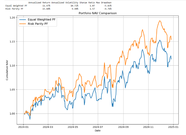
• Danger Parity outperforms with increased annualized return (15.6% vs. 11.5%), decrease volatility (9.9% vs. 10.7%), higher Sharpe ratio (1.57 vs. 1.07), and smaller max drawdown (-4.8% vs. -5.8%).
• Whereas compelling, Danger Parity will depend on historic volatility, it wants frequent rebalancing, and will underperform in sure market situations.

To get probably the most out of this weblog, it’s useful to be aware of a couple of foundational ideas.

Pre-requisites

First, a stable understanding of Python fundamentals is important. This consists of working with primary programming constructs in addition to libraries incessantly utilized in knowledge evaluation. You may discover these ideas in-depth via Fundamentals of Python Programming.

Because the weblog builds on monetary knowledge dealing with, you’ll additionally have to be snug with inventory market knowledge evaluation. This includes studying how you can acquire market datasets, visualise them successfully, and carry out exploratory evaluation in Python. For this, try Inventory Market Information: Acquiring Information, Visualization & Evaluation in Python.

By masking these stipulations, you’ll be well-prepared to dive into the ideas mentioned on this weblog and apply them with confidence.

Desk of contents

Ever puzzled the place your portfolio’s threat is coming from?

Most traders focus closely on selecting the correct shares or funds, however what if the approach you allocate your capital is extra essential than the belongings themselves? Analysis persistently exhibits that asset allocation is the important thing driver of long-term portfolio efficiency. For instance, Vanguard has printed a number of papers reinforcing that asset allocation is the dominant think about portfolio efficiency.

On this publish, we take a more in-depth have a look at Danger Parity, a wise and systematic strategy to portfolio building that goals to stability threat, not simply capital. As a substitute of letting one asset class dominate your portfolio’s threat, Danger Parity spreads publicity extra evenly, doubtlessly resulting in higher stability throughout market cycles.

Quantitative Portfolio Administration is a 3-step course of.

1. Asset choice
2. Asset Allocation
3. Portfolio rebalance and monitoring

In trendy portfolio principle, analysis has proven that “Asset Allocation” has performed a significant function in portfolio efficiency. We’ll perceive Asset Allocation in-depth after which transfer to understanding one of many potential methods to allocate belongings, the Hierarchical Danger Parity methodology.

What’s Asset Allocation?

Allow us to take an instance of a novice investor. This investor has a portfolio of 5 shares and has invested $30,000 in them.

How he/she purchased particular proportions of the shares might rely on subjective evaluation or on the funds they’ve now to purchase shares. And this results in a random publicity of various shares. As given beneath, let’s assume that the novice investor is shopping for shares, and that is how the allocation seems to be:

Notice: A number of the numbers beneath may very well be approximations, for demonstration functions.

Consequently, the proportion of every inventory purchased would extensively differ.

Notice: The variety of shares just isn’t a complete quantity. The calculations are approximations just for demonstration functions.

We clearly see that NVDA has a considerably increased weightage of 39% whereas APPL has merely a weightage of 6%. There’s a nice disparity within the allocation of funds throughout the totally different shares.

Case 1: NVDA underperforms; it is going to have a big affect in your portfolio. Which might result in massive drawdowns, and that is excessive idiosyncratic threat.

Case 2: APPL outperforms, because of a a lot decrease weightage of the inventory in your portfolio. You gained’t profit from it.

How Can We Resolve This Allocation Imbalance?

Quantitative Portfolio Managers don’t allocate funds based mostly on subjectivity. It’s business apply to undertake logical, examined, and efficient methods to do it.

Uneven fund allocation can expose your portfolio to concentrated dangers. To deal with this, a number of systematic asset allocation methods have been developed. Let’s discover probably the most notable ones:

1. Equal Weighting:

Method: Assigns equal capital to every asset.

Notice: The variety of shares just isn’t a complete quantity. The calculations are approximations just for demonstration functions.

• Professionals: Easy, intuitive, and reduces focus threat.
• Cons: Ignores variations in volatility or asset correlation. Could overexpose to riskier belongings.

Actual world instance: MSCI World Equal Weighted Index

2. Imply-Variance Optimisation (MVO)

Method: Primarily based on Trendy Portfolio Concept, it goals to maximise anticipated return for a given degree of threat. Although it seems to be easy, this strategy is adopted by a number of fund managers; its effectiveness comes with periodically rebalancing the portfolio exposures :

1. Anticipated returns
2. Asset volatilities
3. Covariances between belongings

Notice: The variety of shares just isn’t a complete quantity. The calculations are approximations just for demonstration functions.

Monte Carlo simulation is commonly used to check portfolio robustness throughout totally different market situations. To grasp this methodology higher, please learn Portfolio Optimisation Utilizing Monte Carlo Simulation.

The plot beneath exhibits an instance of how portfolios with totally different anticipated returns and volatilities are created utilizing the Monte Carlo Simulation methodology. Hundreds, if no more, mixtures of weights are thought of on this course of. The portfolio weights with the very best Sharpe ratio (marked as +) are sometimes taken because the portfolio with probably the most optimum weightages.

Notice: That is just for demonstration functions, not for shares used for our instance.

• Professionals: Theoretically optimum: When inputs are correct, MVO can assemble probably the most environment friendly portfolio on the risk-return frontier.
• Cons: Extremely delicate to enter assumptions, particularly anticipated returns, that are tough to forecast.

3. Danger-Primarily based Allocation: Danger Parity

Method: As a substitute of allocating capital equally or based mostly on returns, Danger Parity allocates based mostly on threat contribution from every asset. The objective is for every asset to contribute equally to the whole portfolio volatility. The method to attain this consists of the next steps.

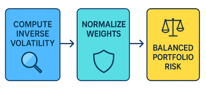
1. Estimate every asset’s volatility
2. Compute the inverse of volatility (i.e., decrease volatility → increased weight).
3. Normalise the inverse of volatility to get last weights.

What’s volatility?

Volatility refers back to the diploma of variation within the worth of a monetary instrument over time. It represents the velocity and magnitude of worth adjustments, and is commonly used as a measure of threat.

In easy phrases, increased volatility means higher worth fluctuations, which may suggest extra threat or extra alternative.

System for Customary Deviation:

$$sigma = sqrt{frac{1}{N-1}sum_{i=1}^N (r_i – bar{r})^2}$$

[
begin{aligned}
text{where,}
&bullet sigma = text{Standard deviation}
&bullet r_i = text{Return at time } i
&bullet bar{r} = text{Average return}
&bullet N = text{Number of periods}
end{aligned}
]

Inverse of Volatility:

The inverse of volatility is solely the reciprocal of volatility. It’s typically used as a measure of risk-adjusted publicity or to allocate weights inversely proportional to threat in portfolio building.

σ=Volatility

Then the Inverse of Volatility is:  1/σ

Normalise the inverse of volatility to get last weights :

To find out the ultimate portfolio weights, we take the inverse of every asset’s volatility after which normalise these values in order that their sum equals 1. This ensures belongings with decrease volatility obtain increased weights whereas sustaining a completely allotted portfolio.

[
w_i = frac{tfrac{1}{sigma_i}}{sum_{j=1}^N tfrac{1}{sigma_j}}
]
$$
textual content{The place,}
bullet w_i quad textual content{= weight of asset $i$ within the portfolio}
bullet sigma_i quad textual content{= volatility (commonplace deviation of returns) of asset $i$}
bullet N quad textual content{= whole variety of belongings within the portfolio}
bullet sum_{j=1}^N tfrac{1}{sigma_j} quad textual content{= sum of the inverse volatilities of all belongings}
$$

Instance of Danger Parity weighted strategy(making use of the above strategy):

The variety of shares just isn’t a complete quantity. The calculations are approximations just for demonstration functions.

Outcome: No single asset dominates the portfolio threat.

Notice:

• Volatility is an instance based mostly on an assumed % commonplace deviation.
• “Danger Parity Weight” is proportional to 1 / volatility, normalised to 100%.
  The publicity is calculated as: Danger Parity Weight × Whole Capital.
• Shares = Publicity ÷ Worth.

Professionals:

• Doesn’t depend on anticipated returns.
• Easy, strong, and makes use of observable inputs.
• Reduces portfolio drawdowns throughout risky intervals.

Cons:

• Could obese low-volatility belongings (e.g., bonds), underweight progress belongings.
• Ignores correlations between belongings (not like HRP).

Different Allocation Strategies to Know:

Danger Parity Allocations Course of in Python

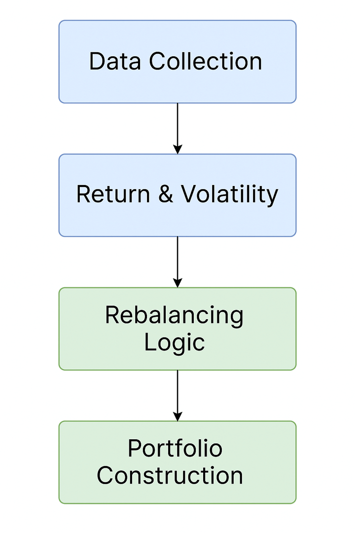
Step 1: Let’s begin by importing the related libraries

Step 2: We fetch the information for 30 shares utilizing their Yahoo Finance ticker symbols.

• These 30 shares are the present 30 constituents of the Dow Jones Industrial Common Index.
• We fetch the information from one month earlier than 2024 begins. And goal a window of the whole yr 2024. That is achieved as a result of we use a 20-day rolling interval to compute volatilities and rebalance the portfolios. 20 buying and selling days roughly interprets to at least one month.
• Solely the “Shut” costs are extracted, and the information body is flattened for additional evaluation.

Step 3: We create a operate to compute the returns of portfolios which can be both equally weighted or weighted utilizing the Danger Parity strategy.

Goal: To compute a portfolio’s cumulative NAV (Internet Asset Worth) utilizing equal-weighted or risk-parity rebalancing at mounted intervals.

• price_df: DataFrame containing historic worth knowledge of a number of belongings, listed by date.
• rebalance_period (default = 20):
  Variety of buying and selling days between every portfolio rebalancing.
• methodology (default=”equal”):
  Portfolio weighting methodology – both ‘equal’ for equal weights or ‘risk_parity’ for inverse volatility weights.

Step-by-Step Logic

• Every day Returns Calculation: The operate begins by computing each day returns utilizing pct_change() on the value knowledge and dropping the primary NaN row.

• Rolling Volatility Estimation: A rolling commonplace deviation is computed over the rebalance window to estimate asset volatility. To keep away from look-ahead bias, that is shifted by sooner or later utilizing .shift(1).

• Begin Alignment: The earliest date all rolling volatility is offered is recognized. The returns and volatility DataFrames are trimmed accordingly.

• NAV Initialisation: A brand new Sequence is created to retailer the portfolio NAV, initialised at 1.0 on the primary legitimate date.

• Rebalance Loop: The operate loops via the information in home windows of rebalance_period days:

• Volatility and Weights on Rebalance Day: On the primary day of every window:

• Cumulative Returns & NAV Computation: The window’s cumulative returns are calculated and mixed with weights to compute the NAV path.

• NAV Normalisation: The NAV is normalised to match the final worth of the earlier window, making certain easy continuity.

Closing Output: Returns a time collection of the portfolio’s NAV, excluding any lacking values.

Step 4: Portfolio Building

We now proceed to assemble two portfolios utilizing the historic worth knowledge. This includes calling the portfolio building operate outlined earlier. Particularly, we generate:

1. An Equal-Weighted Portfolio, the place every asset is assigned the identical weight at each rebalancing interval.
2. A Danger Parity Portfolio, the place asset weights are decided based mostly on inverse volatility, aiming to equalise threat contribution throughout all holdings.

Each portfolios are rebalanced periodically based mostly on the desired frequency.

Step 5: Portfolio Efficiency Analysis

On this step, we consider the efficiency of the 2 constructed portfolios: Equal-Weighted and Danger Parity, by computing key efficiency metrics:

• Every day Returns: Calculated from the cumulative NAV collection to look at day-to-day efficiency fluctuations.
• Annualised Return: Derived utilizing the compound return over the whole funding interval, scaled to replicate yearly efficiency.
• Annualised Volatility: Estimated from the usual deviation of each day returns and scaled by the sq. root of 252 buying and selling days to annualise.
• Sharpe Ratio: A measure of risk-adjusted return, computed because the ratio of annualised return to annualised volatility, assuming a risk-free price of 0.
• Most Drawdown: The utmost noticed peak-to-trough decline in portfolio worth, indicating the worst-case historic loss.

These metrics provide a complete view of how every portfolio performs when it comes to each return and threat. We additionally visualise the cumulative NAVs of each portfolios to look at their efficiency developments over time.

Continuously Requested Questions

What precisely is Danger Parity?

Danger Parity is a portfolio allocation technique that assigns weights such that every asset contributes equally to the whole portfolio volatility, moderately than merely allocating equal capital to every asset. The objective is to stop any single asset or asset class from dominating the portfolio’s general threat publicity.

How does it differ from Equal Weighting or Imply-Variance Optimisation?

• Equal Weighting: This methodology allocates the identical quantity of capital to every asset. It’s easy and intuitive, however doesn’t contemplate the danger (volatility) of every asset, doubtlessly resulting in concentrated threat.
• Imply-Variance Optimisation (MVO): Primarily based on Trendy Portfolio Concept, MVO seeks to maximise anticipated return for a given degree of threat by contemplating anticipated returns and covariances. Nevertheless, it’s extremely delicate to the accuracy of enter forecasts.
• Danger Parity: As a substitute of specializing in returns or allocating equal capital, Danger Parity adjusts weights based mostly on the volatility of every asset, allocating extra capital to lower-volatility belongings to equalise their threat contributions.

Why is asset allocation so essential?

Analysis has proven that asset allocation is the first driver of long-term portfolio returns, much more vital than choosing particular person securities. A well-thought-out allocation helps handle threat and enhances the probability of assembly funding targets.

How is volatility calculated in Danger Parity?

Volatility is usually measured as the usual deviation of previous returns over a rolling window (for instance, a 20-day rolling commonplace deviation). In Danger Parity, belongings with decrease volatility are assigned increased weights to stability their contribution to whole portfolio threat.

Is there Python code to implement this?

Sure. The weblog supplies full Python code examples utilizing libraries similar to pandas for knowledge dealing with, yfinance for fetching historic costs, and customized capabilities to rebalance portfolios both by equal weights or by inverse volatility (Danger Parity).

Does Danger Parity at all times outperform different methods?

No. Whereas Danger Parity typically results in extra secure efficiency and higher risk-adjusted returns, particularly in diversified or risky markets, it might underperform less complicated methods like Equal-Weighted portfolios throughout sturdy bull markets that favour high-risk belongings.

What are the restrictions of Danger Parity?

• It depends on the historic volatility to set goal weights, which can not precisely replicate  the longer term behaviour of belongings, particularly throughout abrupt adjustments or crises.
• It sometimes requires frequent rebalancing, which may improve transaction prices and potential slippage.
• It could under-allocate to high-growth belongings in trending markets, limiting upside in sturdy rallies.

Are there extra superior strategies past commonplace Danger Parity?

Sure. For instance, Hierarchical Danger Parity (HRP) makes use of clustering to know asset relationships and goals to allocate threat extra effectively by addressing a few of the weaknesses of conventional mean-variance approaches, similar to instability because of enter sensitivity.

Conclusion

The comparative evaluation highlights the clear benefits of utilizing a Danger Parity strategy over a conventional Equal-Weighted portfolio. Whereas each portfolios ship constructive returns, Danger Parity stands out with:

• Greater Annualised Return (15.60% vs. 11.47%)
• Decrease Volatility (9.90% vs. 10.72%)
• Superior Danger-Adjusted Efficiency, as seen within the Sharpe Ratio (1.57 vs. 1.07)
• Smaller Max Drawdown (-4.76% vs. -5.83%)

These outcomes reveal that by aligning portfolio weights with asset threat (moderately than capital), the Danger Parity portfolio could improve return potential together with higher draw back safety and smoother efficiency over time.

The NAV chart additional reinforces this conclusion, exhibiting a extra constant and resilient progress trajectory for the Danger Parity technique.

In abstract, for traders prioritising stability over progress, Danger Parity presents a compelling various to traditional allocation strategies.

A Notice on Limitations

Though the Danger Parity portfolio delivered stronger returns throughout the interval taken in our instance, its efficiency benefit just isn’t assured in each market section. Like several technique, Danger Parity comes with limitations. It depends closely on historic volatility estimates, which can not at all times precisely replicate future market situations, particularly throughout sudden regime shifts or excessive occasions.

It tends to shine in portfolios that blend excessive‑ and low‑volatility belongings, like shares and bonds, the place equal capital allocation would in any other case focus threat.Nevertheless, if low‑volatility belongings underperform or if all belongings have related threat profiles,

Moreover, the technique typically requires frequent rebalancing, which may improve transaction prices and introduce slippage. In sturdy directional markets, notably these favouring higher-risk belongings, less complicated methods like Equal-Weighted could outperform because of their higher publicity to momentum.

Therefore, whereas Danger Parity supplies a scientific option to stability portfolio threat, it needs to be used with an understanding of its assumptions and sensible limitations.

Subsequent Steps:

After studying this weblog, you might wish to improve your understanding of portfolio design and discover strategies that present extra construction to risk-return trade-offs.

A very good place to start is with Portfolio Variance/Covariance Evaluation, which explains how asset correlations affect portfolio volatility. It will offer you the muse to know why diversification works and the place it doesn’t.

From there, Portfolio Optimisation Utilizing Monte Carlo Simulation introduces a extra dynamic strategy. By operating 1000’s of simulated outcomes, you possibly can take a look at how totally different allocations behave below uncertainty and determine mixtures that stability threat and reward.

To spherical it off, Portfolio Optimisation Strategies walks via a variety of optimisation frameworks, masking classical mean-variance fashions in addition to various strategies, so you possibly can evaluate their strengths and apply them in several market situations.

Working via these subsequent steps will equip you with sensible strategies to analyse, simulate, and optimise portfolios, a ability set that’s crucial for anybody trying to handle capital with confidence.

You may discover all of those intimately within the Portfolio Administration & Place Sizing Studying Monitor, which incorporates the Quantitative Portfolio Administration course for a complete understanding of portfolio building and optimisation.

For these trying to broaden past portfolio principle into the broader realm of systematic buying and selling, examine the Govt Programme in  Algorithmic Buying and selling – EPAT. Its complete curriculum, led by high college like Dr. Ernest P. Chan, presents a number one Python algorithmic buying and selling course for profession progress. EPAT covers core buying and selling methods that may be tailored and prolonged to Excessive-Frequency Buying and selling. Get personalised assist for specialising in buying and selling methods with reside venture mentorship.

Disclaimer: This weblog publish is for informational and academic functions solely. It doesn’t represent monetary recommendation or a suggestion to commerce any particular belongings or make use of any particular technique. All buying and selling and funding actions contain vital threat. All the time conduct your personal thorough analysis, consider your private threat tolerance, and contemplate in search of recommendation from a certified monetary skilled earlier than making any funding selections.