

By Rekhit Pachanekar and Ishan Shah
Is it attainable to foretell the place the Gold worth is headed?
Sure, let’s use machine studying regression strategies to foretell the value of probably the most essential treasured metallic, the Gold.
Gold is a key monetary asset and is extensively thought to be a protected haven in periods of financial uncertainty, making it a most popular selection for buyers looking for stability and portfolio diversification.
We’ll create a machine studying linear regression mannequin that takes data from the previous Gold ETF (GLD) costs and returns a Gold worth prediction the subsequent day.
GLD is the biggest ETF to speculate immediately in bodily gold. (Supply)
This mission prioritizes establishing a stable basis with extensively used machine studying strategies as an alternative of instantly turning to superior fashions. The target is to construct a sturdy and scalable pipeline for predicting gold costs, designed to be simply adaptable for incorporating extra subtle algorithms sooner or later.
We’ll cowl the next matters in our journey to foretell gold costs utilizing machine studying in python.
Import the libraries and skim the Gold ETF knowledge
First issues first: import all the required libraries that are required to implement this technique. Importing libraries and knowledge information is an important first step in any knowledge science mission, because it ensures you might have all dependencies and exterior knowledge sources prepared for evaluation.
Then, we learn the previous 14 years of every day Gold ETF worth knowledge from a file and retailer it in Df. This knowledge set features a date column, which is crucial for time collection evaluation and plotting developments over time. We take away the columns which aren’t related and drop NaN values utilizing dropna() perform. Then, we plot the Gold ETF shut worth.
Output:
Outline explanatory variables
An explanatory variable, also referred to as a function or unbiased variable, is used to clarify or predict modifications in one other variable. On this case, it helps predict the next-day worth of the Gold ETF.
These are the inputs or predictors we use in a mannequin to forecast the goal consequence.
On this technique, we begin with two easy options: the 3-day shifting common and the 9-day shifting common of the Gold ETF. These shifting common function smoothed representations of short-term and barely longer-term developments, serving to seize momentum or mean-reversion habits in costs. Earlier than utilizing these options in modeling, we get rid of any lacking values utilizing the .dropna() perform to make sure the dataset is clear and prepared for evaluation. The ultimate function matrix is saved in X.
Nevertheless, that is just the start of the function engineering course of. You’ll be able to prolong X by incorporating extra variables which may enhance the mannequin’s predictive energy. These could embrace:
- Technical indicators reminiscent of RSI (Relative Power Index), MACD (Transferring Common Convergence Divergence), Bollinger Bands, or ATR (Common True Vary).
- Cross-asset options, reminiscent of the value or returns of associated ETFs just like the Gold Miners ETF (GDX) or the Oil ETF (USO), which can affect gold costs by means of macroeconomic or sector-specific linkages.
- Macroeconomic indicators reminiscent of inflation knowledge (CPI), rates of interest, and USD index actions can affect gold costs as a result of gold is perceived as a safe-haven asset throughout occasions of financial uncertainty.
The method of figuring out and establishing such variables known as function engineering. Individually, choosing probably the most related variables for a mannequin is named function choice.
The higher your options replicate significant patterns within the knowledge, the extra correct your forecasts are more likely to be.
Outline dependent variable
The dependent variable, also referred to as the goal variable in machine studying, is the result we goal to foretell. Its worth is assumed to be influenced by the explanatory (or unbiased) variables. Within the context of our technique, the dependent variable is the value of the Gold ETF (GLD) on the next day.
In our dataset, the Shut column accommodates the historic costs of the Gold ETF. This column serves because the goal variable as a result of we’re constructing a mannequin to study patterns from historic options (reminiscent of shifting averages) and use them to foretell future GLD costs. We assign this goal collection to the variable y, which will likely be used throughout mannequin coaching and analysis.
To create the goal variable, we apply the shift(-1) perform to the Shut column. This shifts the value knowledge one step backward, making every row’s goal the subsequent day’s closing worth. This strategy allows the mannequin to make use of as we speak’s options to forecast tomorrow’s worth.
Clearly defining the goal variable is crucial for any supervised studying drawback, because it shapes your entire modelling goal. On this case, the purpose is to forecast future actions in gold costs utilizing related monetary and financial indicators.
Alternatively, as an alternative of predicting absolutely the worth of gold, we are able to use gold returns because the goal variable. Returns characterize the proportion change in gold costs over a specified time interval, reminiscent of every day, weekly, or month-to-month intervals.
Non-stationary variables in linear regression
In time collection evaluation, it is common to work with uncooked monetary knowledge reminiscent of inventory or commodity costs. Nevertheless, these worth collection are usually non-stationary, that means their statistical properties like imply and variance change over time. This poses a major problem as a result of many analytical strategies depend on the idea that the information behaves constantly. When the information is non-stationary, its underlying construction shifts. Traits evolve, volatility varies, and historic patterns could not maintain sooner or later.
Working with non-stationary knowledge can result in a number of issues:
- Spurious Relationships: Variables could look like associated just because they share related developments, not as a result of there is a real connection.
- Unstable Insights: Any patterns or relationships recognized could not maintain over time, as the information’s behaviour continues to evolve.
- Deceptive Forecasts: Predictive fashions constructed on non-stationary knowledge usually battle to carry out reliably sooner or later.
The core challenge is that non-stationary processes don’t comply with mounted guidelines. Their dynamic nature makes it tough to attract conclusions or make predictions that stay legitimate as circumstances change. Earlier than performing any critical evaluation, it is essential to check for stationarity and, if wanted, rework the information to stabilize its behaviour.
Two Methods to Work with Non-Stationary Knowledge
Slightly than discarding non-stationary variables, there are two dependable methods to deal with them in linear regression fashions:
1. Make Variables Stationary (Differencing Strategy)
One widespread technique is to rework the information to make it stationary. That is usually executed by specializing in modifications in values. For instance, worth collection may be transformed into returns or variations. This transformation helps stabilize the imply and reduces developments or seasonality. As soon as the information is reworked, it turns into extra appropriate for linear modeling as a result of its statistical properties stay constant over time.
2. Use Unique Non-Stationary Sequence (Cointegration Strategy)
The second technique permits us to make use of the unique non-stationary collection with out transformation, offered sure circumstances are met. Particularly, it entails checking whether or not the variables, when mixed in a selected means, share a long-term equilibrium relationship. This idea is named cointegration.
Even when the person variables are non-stationary, their linear mixture may be stationary. If that is so, the residuals from the regression (the variations between precise and predicted values) stay steady over time. This stability makes the regression legitimate and significant, because it displays a real relationship somewhat than a statistical coincidence.
In our evaluation, we are going to use this second technique by testing for residual stationarity to verify that the regression setup is suitable.
Output:
Cointegration p-value between S_3 and next_day_price: 3.1342217460742354e-16
Cointegration p-value between S_9 and next_day_price: 1.268049574487298e-15
S_3 and next_day_price are cointegrated.
S_9 and next_day_price are cointegrated.
The time collection S_3 (3-day shifting common) and next_day_price, in addition to S_9 (9-day shifting common) and next_day_price, are cointegrated. Thus, we are able to proceed with working a linear regression immediately with out reworking the collection to attain stationarity.
Why You Can Run the Regression Immediately?
Cointegration implies that there’s a steady, long-term relationship between the 2 non-stationary collection. Which means whereas the person collection could every include unit roots (i.e., be non-stationary), their linear mixture is stationary and working an Abnormal Least Squares (OLS) regression is not going to result in a spurious regression. It is because the residuals of the regression (i.e., the distinction between the expected and precise values) will likely be stationary.
Key Factors to Bear in mind
As cointegration already ensures a sound statistical relationship, making OLS acceptable for estimating the parameters, there isn’t a have to distinction the collection to make them stationary earlier than working the regression
The regression run between S_3 (or S_9) and next_day_price will seize a sound long-term equilibrium relationship, which cointegration confirms.
Cut up the information into practice and take a look at dataset
On this step, we break up the predictors and output knowledge into practice and take a look at knowledge. The coaching knowledge is used to create the linear regression mannequin, by pairing the enter with anticipated output.
Mannequin coaching is carried out on the coaching dataset, the place the mannequin learns from the options and labels.
The take a look at knowledge is used to estimate how properly the mannequin has been skilled. Evaluating completely different fashions and evaluating their coaching time and accuracy is a crucial a part of the mannequin choice course of. Mannequin analysis, together with the usage of validation units and cross-validation, ensures the mannequin generalizes properly to unseen knowledge.
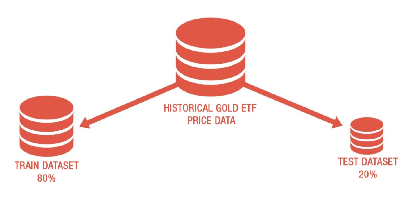
- First 80% of the information is used for coaching and remaining knowledge for testing
- X_train & y_train are coaching dataset
- X_test & y_test are take a look at dataset
Create a linear regression mannequin
We’ll now create a linear regression mannequin. However, what’s linear regression?
Linear regression is likely one of the easiest and most generally used algorithms in machine studying for supervised studying duties, the place the purpose is to foretell a steady goal variable based mostly on enter options. At its core, linear regression captures a mathematical relationship between the unbiased variables (x) and the dependent variable (y) by becoming a straight line that finest describes how modifications in x have an effect on the values of y.
When the information is plotted as a scatter plot, linear regression identifies the road that minimizes the distinction between the precise values and the expected values. This fitted line represents the regression equation and is used to make future predictions.
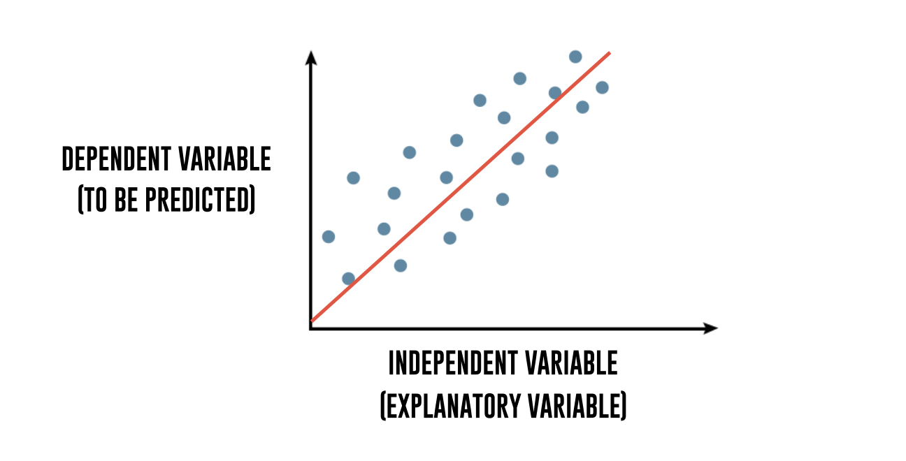
To interrupt it down additional, regression explains the variation in a dependent variable when it comes to unbiased variables. The dependent variable – ‘y’ is the variable that you just need to predict. The unbiased variables – ‘x’ are the explanatory variables that you just use to foretell the dependent variable. The next regression equation describes that relation:
Y = m1 * X1 + m2 * X2 + C
Gold ETF worth = m1 * 3 days shifting common + m2 * 9 days shifting common + c
Then we use the match technique to suit the unbiased and dependent variables (x’s and y’s) to generate coefficient and fixed for regression.
Output:
Linear Regression mannequin
Gold ETF Value (y) = 1.19 * 3 Days Transferring Common (x1) + -0.19 * 9 Days Transferring Common (x2) + 0.28 (fixed)
Predict the Gold ETF costs
Now, it’s time to examine if the mannequin works within the take a look at dataset. We predict the Gold ETF costs utilizing the linear mannequin created utilizing the practice dataset. The predict technique finds the Gold ETF worth (y) for the given explanatory variable X.
Output:
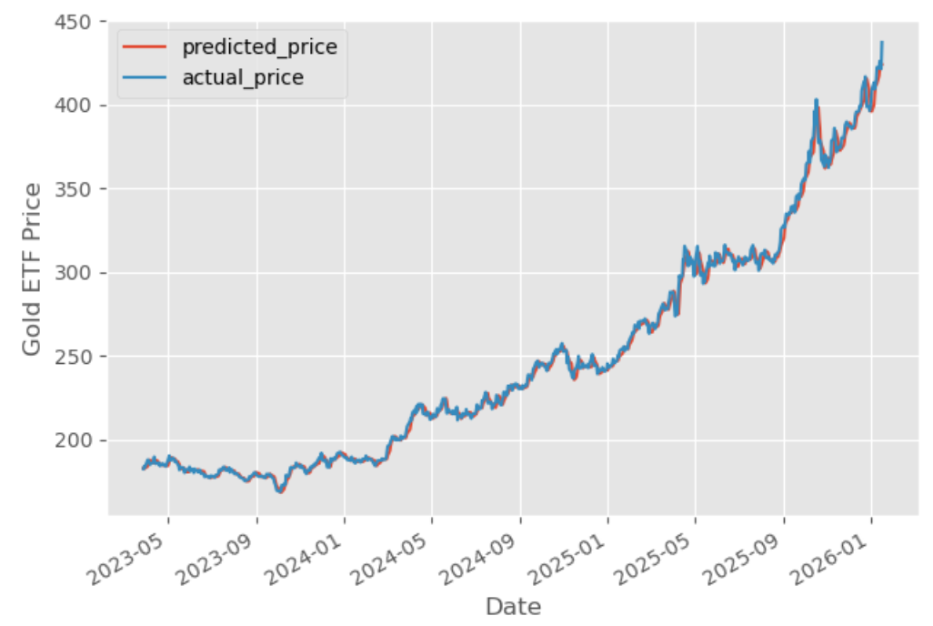
The graph exhibits the expected costs and precise costs of the Gold ETF. Evaluating predicted costs to precise costs helps consider the efficiency of the skilled mannequin and exhibits how carefully the predictions match real-world values. Capabilities like evaluate_model() can be utilized to generate diagnostic plots and additional consider the mannequin’s high quality.
Now, let’s compute the goodness of the match utilizing the rating() perform.
Output:
99.70
As it may be seen, the R-squared of the mannequin is 99.70%. R-squared is at all times between 0 and 100%. A rating near 100% signifies that the mannequin explains the Gold ETF costs properly.
On the floor, this appears spectacular. It exhibits a near-perfect match between the mannequin’s outputs and actual market values.
Nevertheless, translating this predictive accuracy right into a worthwhile buying and selling technique just isn’t simple. In follow, it’s essential make vital choices reminiscent of:
- When to enter a commerce (sign era)
- How lengthy to maintain the place
- When to exit (e.g., based mostly on a predicted reversal or mounted threshold)
- And the right way to handle threat (e.g., utilizing stop-loss or place sizing)
As an instance this problem, we tried to make use of predicted costs to generate a easy long-only buying and selling sign.
A place is taken provided that the subsequent day’s predicted worth is greater than as we speak’s closing worth. This creates a unidirectional sign with no shorting or hedging. The place is exited (and doubtlessly re-entered) each time the sign situation is not met.
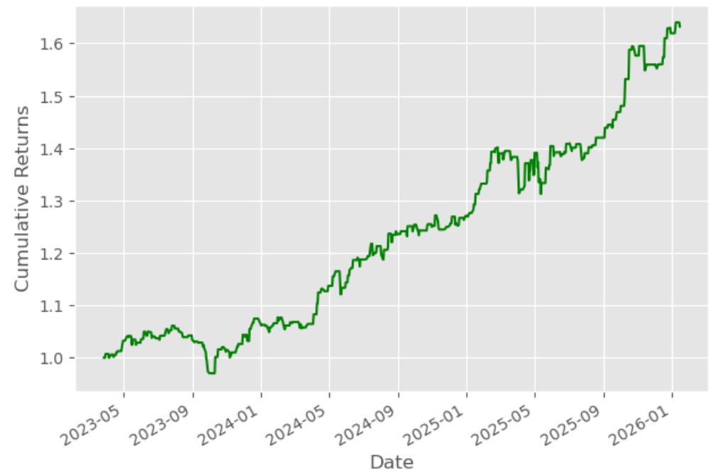
Plotting cumulative returns
Let’s calculate the cumulative returns of this technique to analyse its efficiency.
- The steps to calculate the cumulative returns are as follows:
- Generate every day share change of gold worth
- Shift the every day share change forward by in the future to align with our place when there’s a sign.
- Create a purchase buying and selling sign represented by “1” when the subsequent day’s predicted worth is greater than the present day worth. No place is taken in any other case
- Calculate the technique returns by multiplying the every day share change with the buying and selling sign.
- Lastly, we are going to plot the cumulative returns graph
The output is given beneath:
We may even calculate the Sharpe ratio.
The output is given beneath:
‘Sharpe Ratio 1.82′
Given the mannequin’s excessive predictive accuracy, the Sharpe Ratio of the ensuing buying and selling technique is just one.82, which isn’t excellent for a scalable and sensible buying and selling system.
This disparity highlights a vital level: good worth prediction doesn’t at all times result in extraordinarily worthwhile or risk-adjusted buying and selling efficiency. A number of components could clarify the decrease Sharpe Ratio:
The technique could endure from unidirectional bias, ignoring shorting or range-bound intervals.
- It may not adapt properly to market volatility, resulting in sharp drawdowns.
- The buying and selling guidelines are too simplistic, failing to seize timing nuances or noise within the predictions.
In abstract, whereas the mannequin performs properly in predicting worth ranges, changing this into a sturdy buying and selling technique requires considerate design. Sign logic, timing, place administration, and threat controls all play a major position in enhancing precise technique efficiency.
Steered Reads:
Tips on how to use this mannequin to foretell every day strikes?
You need to use the next code to foretell the gold costs and provides a buying and selling sign whether or not we should always purchase GLD or take no place.
The output is as proven beneath:
| Date | 2026-01-20 |
|---|---|
| Value | |
| Shut | 437.230011 |
| sign | No Place |
| predicted_gold_price | 427.961362 |
Congrats! You’ve got simply applied a easy but efficient machine studyingmethod utilizing linear regression to forecast gold costs and derive buying and selling indicators. You now perceive the right way to:
- Engineer options from uncooked worth knowledge (utilizing shifting averages),
- Construct and match a predictive mannequin,
- Use the mannequin for making forward-looking forecasts,and
- Translate these forecasts into actionable indicators.
What’s Subsequent?
Linear regression is a superb place to begin resulting from its simplicity and interpretability. However in real-world monetary modeling,extra complicated patterns and nonlinear relationships usually exist that linear fashions may not absolutely seize.
To enhance accuracy,you’ll be able to discover extra highly effective machine studying regression fashions,reminiscent of:
- Random Forest Regression
- Gradient Boosted Bushes (like XGBoost or LightGBM)
- Assist Vector Regression (SVR)
- Neural Networks (MLPs for tabular knowledge)
The core construction of your pipeline stays the identical:knowledge preprocessing,function engineering,forecasting,and sign era. The one change is the mannequin itself. You merely change the .match() and .predict() strategies with these out of your chosen algorithm,probably adjusting a number of extra hyperparameters.
Hold Exploring
Wish to dive deeper into utilizing machine studying for buying and selling? Be taught step-by-step the right way to construct your first ML-based buying and selling technique with our guidedcourse. When you’re able to take it to the subsequent stage,discover our Studying Monitor. Consultants like Dr. Ernest Chan will information you thru your entire lifecycle,from concept era and backtesting to dwell deployment,utilizing superior machine studying strategies.
File within the obtain:
Gold Value Prediction Technique –Python Pocket book
Disclaimer:All investments and buying and selling within the inventory market contain threat. Any choices to put trades within the monetary markets,together with buying and selling in inventory or choices or different monetary devices is a private resolution that ought to solely be made after thorough analysis,together with a private threat and monetary evaluation and the engagement{of professional}help to the extent you consider needed. The buying and selling methods or associated data talked about on this article is for informational functions solely.