Stata 15 introduced, accessible now

We introduced Stata 15 right this moment. It’s a giant deal as a result of that is Stata’s largest launch ever.

I posted to Statalist this morning and listed sixteen of an important new options. Right here on the weblog I’ll say extra about them, and you’ll be taught much more by visiting our web site and seeing the Stata 15 options web page.

I’m going into depth under on the sixteen highlighted options. They’re (click on to leap)

 

1. Prolonged regression fashions
2. Latent class evaluation (LCA)
3. Bayesian prefix command
4. Linearized dynamic stochastic basic equilibrium (DSGE) fashions
5. Dynamic Markdown paperwork for the net
6. Nonlinear mixed-effects fashions
7. Spatial autoregressive fashions (SAR)
8. Interval-censored parametric survival-time fashions
9. Finite combination fashions (FMMs)
10. Combined logit fashions
11. Nonparametric regression
12. Energy evaluation for cluster randomized designs and regression fashions
13. Phrase and PDF paperwork
14. Graph coloration transparency/opacity
15. ICD-10-CM/PCS help
16. Federal Reserve Financial Information (FRED) help
17. And extra

The sixteen options listed above actually necessary ones, however there are others worthy of point out. Extra come readily to thoughts:

• Bayesian multilevel fashions
• Threshold regression
• Panel-data tobit with random coefficients
• Multilevel regression for interval-measured outcomes
• Multilevel tobit regression for censored outcomes
• Panel knowledge cointegration assessments
• Checks for a number of breaks in time sequence
• A number of-group generalized SEM
• Heteroskedastic linear regression
• Poisson fashions with Heckman-style pattern choice
• Panel-data nonlinear fashions with random coefficients
• Bayesian panel-data fashions
• Panel-data interval regression with random coefficients
• SVG export
• Bayesian survival fashions
• Zero-inflated ordered probit
• Add your individual energy and sample-size strategies
• Bayesian sample-selection fashions
• Stata in Swedish
• Enhancements to the Do-file Editor
• Stream random-number generator
• Enhancements for Java plugins
• Extra parallelization in Stata/MP

 

1. Prolonged regression fashions

We name them ERMs—prolonged regression fashions. 4 new instructions match

• linear regressions,
• interval regressions together with tobit,
• probit, and
• ordered probit fashions

with any mixture of

• endogenous covariates,
• nonrandom remedy task, and
• endogenous (Heckman-style) pattern choice.

These new instructions are simply wanting superb as a result of you possibly can put endogenous covariates in any of the equations, and that features the treatment-assignment and probit-selection equations. And endogenous covariates are usually not restricted to being steady. They are often binary or ordinal. And they are often interacted with different covariates, whether or not exogenous or endogenous. They will even be interacted with themselves to type squared or cubic phrases!

These new ERM instructions—eregress, eintreg, eprobit, and eoprobit—are destined to turn into in style as a result of they tackle so lots of the issues researchers have. First, you may need an endogenous variable as a result of a lot of fashions have omitted variables which are correlated with the variables within the mannequin. Subsequent, knowledge are sometimes censored, and the censoring is just not random. ERM sample-selection choices let you mannequin the sample-selection course of and so regulate for it. Or if you’re becoming a treatment-effects mannequin with nonrandom task, you should utilize ERM treatment-assignment choices. Or you possibly can mix the treatment-assignment and choice choices, which will likely be of particular curiosity to these becoming endogenous treatment-assignment fashions wherein some are misplaced due to follow-up.

The syntax is easy:

. eregress   y x1 x2

. eregress   y x1 x2,  endogenous(       x2 = x3 x4, nomain)

. eregress   y x1 x2,  endogenous(       x2 = x3 x4, nomain) 
                           choose( chosen = x2 x5)          

. eregress   y x1 x2,  endogenous(       x2 = x3 x4, nomain) 
                          entreat(  handled = x2 x5)          

. eregress   y x1 x2,  endogenous(      x2 = x3 x5, nomain)
                          entreat( handled = x2 x3 x4)          
                           choose(chosen = x2 x6)          

eregress matches linear regressions. You’ll be able to simply as simply match a probit mannequin as a linear regression mannequin. If the end result variable y is binary, sort

. eprobit    y x1 x2,  endogenous(      x2 = x3 x5, nomain)
                          entreat( handled = x2 x3 x4)
                           choose(chosen = x2 x6) 

If the end result variable y is steady however the variable x2 is binary, sort

. eregress   y x1 x2,  endogenous(     x2 = x3 x5, binary nomain)
                         entreat( handled = x2 x3 x4) 
                          choose(chosen = x2 x6)  

If each y and x2 are binary, sort

. eprobit    y x1 x2,  endogenous(     x2 = x3 x5, binary nomain)
                         entreat( handled = x2 x3 x4) 
                          choose(chosen = x2 x6)  

In case you’re questioning in regards to the unusual nomain choice, it’s a element. Once you specify endogenous(title=…), variable title is added to the principle equation mechanically. You’ll be able to sort

. eregress y x1,     endogenous(x2=x3 x4)

or

. eregress y x1 x2,  endogenous(x2=x3 x4, nomain)

and, both manner, the identical mannequin is match. I specified nomain within the opening examples simply so I’d not have to elucidate that the choice included x2 in the principle equation.

See the examples on the Stata 15 ERMs web page.

Again to highlights.

 

2. Latent class evaluation (LCA)

Latent means unobserved. Class means group. Latent lessons are unobserved teams inside your knowledge. You may need knowledge on shoppers and imagine they’re divided into three teams relying on their potential curiosity in your product. Sadly, you would not have variables within the knowledge specifying the group to which every client belongs. When you’ve got 4 binary variables which are indicators of the latent class to which shoppers belong, nonetheless, you possibly can sort

. gsem (y1 y2 y3 y4 <- cons), lclass(Consum 3) logit

y1, y2, y3, and y4 are noticed. Consum is the latent categorical variable that lclass(Consum 3) specified as taking over three values. The result’s to suit a mannequin wherein y1, y2, y3, and y4 are decided by unobserved class.

The command matches 4x3=12 logistic regressions, one for every of the 4 y variables and every of the three lessons. Every regression has an intercept. As well as, a multinomial logistic regression can be match to foretell Consum.

After becoming the mannequin, you possibly can

• use the brand new estat lcprob command to estimate the proportion of shoppers belonging to every class;
• use the brand new estat lcmean command to estimate the marginal technique of y1, y2, y3, and y4 in every class (the means will likely be possibilities for the instance proven);
• use the brand new estat lcgof command to guage the goodness of match; and
• use the prevailing predict command to acquire predicted possibilities of sophistication membership and predicted values of noticed consequence variables.

See extra on the Stata 15 Latent class evaluation web page.

Again to highlights.

 

3. Bayesian prefix command

The brand new bayes: prefix command allows you to match a wider vary of Bayesian fashions than have been beforehand accessible. You all the time may match a Bayesian linear regression, however now you possibly can match it by typing

. bayes: regress y x1 x2 

That’s handy. What you may not beforehand do was match a Bayesian survival mannequin. Now you possibly can:

. bayes: streg x1 x2, distribution(weibull) 

You’ll be able to even match Bayesian multilevel survival fashions:

. bayes: streg x1 x2 || id:, distribution(weibull)

On this mannequin, random intercepts have been added for every worth of variable id.

The brand new bayes: prefix command works in entrance of many Stata estimation instructions that present over 50 chance fashions. See the complete record right here. Among the many supported fashions are multilevel, panel knowledge, survival, and sample-selection fashions!

All of Stata’s Bayesian options are supported by the brand new command. You’ll be able to choose from prior distributions for mannequin parameters, or use default priors. You should utilize the default adaptive Metropolis–Hastings sampling, or Gibbs sampling, or a mix of the 2 strategies, when closed-form options can be found for the Gibbs methodology. And you should utilize another function of Stata’s underlying bayesmh command. You would change the default prior distributions for the regression coefficients, for example, utilizing the prior() choice:

. bayes, prior({y: x1 x2}, regular(0,4)): regress y x1 x2

After estimation, you should utilize Stata’s customary Bayesian postestimation instruments corresponding to

• bayesgraph to test convergence,
• bayesstats abstract to estimate capabilities of mannequin parameters,
• bayesstats ic and bayestest mannequin to compute Bayes elements and examine Bayesian fashions, and
• bayestest interval to carry out interval hypotheses testing.

See extra on the Stata 15 Bayesian estimation web page.

Again to highlights.

 

4. Linearized dynamic stochastic basic equilibrium (DSGE) fashions

DSGEs are a time-series mannequin utilized in economics. They’re options to conventional forecasting fashions. Each try to elucidate combination financial phenomena, however DSGEs permit doing this on the idea of fashions derived from financial concept.

Being primarily based on financial concept means a lot of equations. The important thing function of those equations is that expectations of future variables have an effect on variables right this moment. That is one function that distinguishes DSGEs from a vector autoregression or a state-space mannequin. The opposite function is that, being derived from concept, the parameters can often be interpreted when it comes to that concept.

Right here is the way you match a two-equation DSGE mannequin in Stata. Curly braces, { }, are used to surround the parameters to be match:

. dsge (   p = {beta}*E(f.p) + {kappa}*y )
       ( f.y = {rho}*y, state )

p is a management variable, and y is a state variable in state-space jargon. f. is the ahead operator. Right here is how you can learn them:

1. The primary equation,

   ( p = {beta}*E(f.p) + {kappa}*y )
   

   says that the management variable p is determined by {beta}*p sooner or later plus {kappa}*y right this moment.

2. The second equation,

   ( f.y = {rho}*y, state )
   

   says that the anticipated future worth of y is {rho}*y right this moment. The state choice specifies that y is a state variable.

There are three sorts of variables in DSGE fashions.

• Management variables and equations corresponding to p don’t have any shocks and are decided by the system of equations.
• State variables corresponding to y have implied shocks and are predetermined initially of the time interval.
• Shocks are the stochastic errors that drive the system.

In any case, the above dsge command defines a mannequin and matches it.

If we’ve got a concept in regards to the relationship between beta and kappa corresponding to that they’re equal, we may take a look at it utilizing current command take a look at within the normal manner.

New postestimation instructions estat coverage and estat transition report the coverage and transition matrices. In case you sort

. estat coverage

displayed would be the management variables as a linear perform of the state variables. In case you had 5 management variables and three state variables, every of the controls could be reported as a linear perform of the three states. Within the easy instance above, the linear perform predicting p will likely be proven as a perform of y right this moment.

In the meantime,

. estat transition

reviews the transition matrix. Whereas the coverage matrix reviews p as a perform of y, the transition matrix reviews how y evolves via time unique of p.

You’ll be able to produce forecasts utilizing Stata’s current forecast command. You’ll be able to graph impulse–response capabilities utilizing Stata’s current irf command.

Right here is an impulse–response graph:

See extra on the Stata 15 Linearized DSGEs web page.

Again to highlights.

 

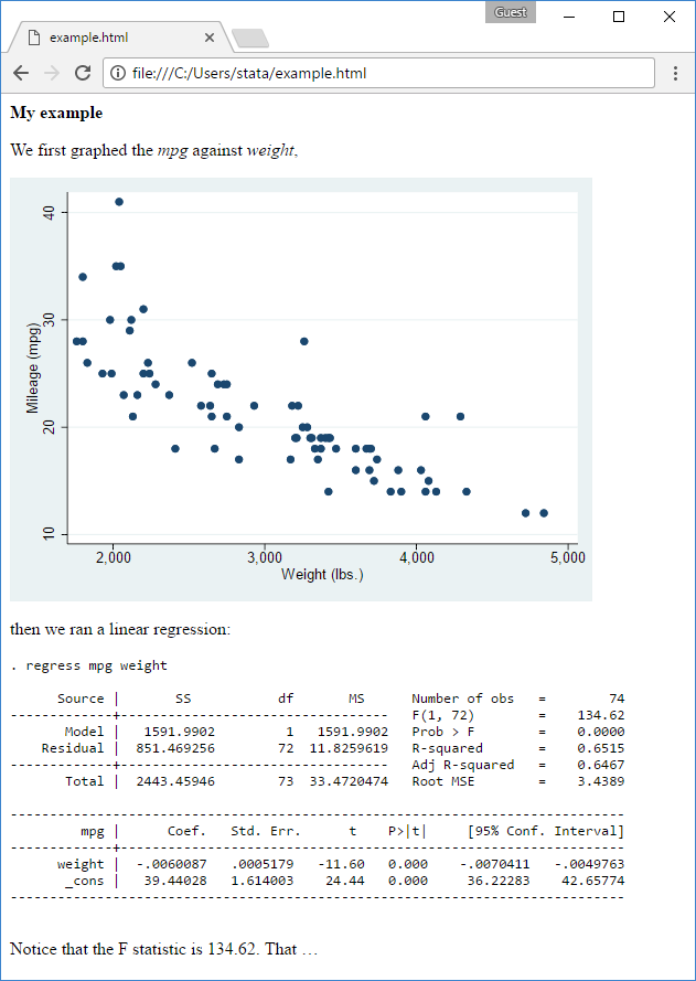
5. Dynamic Markdown paperwork for the net

Have you ever ever heard of Markdown? It’s a in style manner of making HTML paperwork. HTML recordsdata are fiddly. Markdown is easy and intuitive. The concept is easy sufficient. You create a file containing textual content you need with human-readable formatting, and you then run a command to create an HTML file from it.

Stata now helps Markdown, and we’ve got added tags (options) to Markdown that let you embody Stata instructions within the enter file. The instructions you embody will likely be run and displayed, or will likely be run in secret, and components of the output extracted to be used within the doc.

You would possibly create a file corresponding to

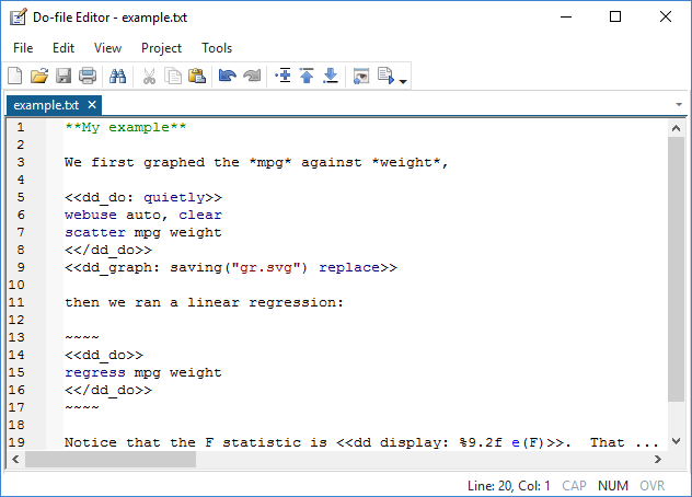
In Stata, you sort

. dyndoc instance.txt

and now you’ve got a brand new file named instance.html that, on the net, seems like this:

Be taught extra in regards to the Markdown language at Wikipedia.

Be taught extra about our implementation at our Stata 15 Markdown & dynamic paperwork web page.

dyndoc, by the best way, stands for dynamic doc. The Markdown file you create is dynamic within the sense that, ought to your knowledge change, you possibly can re-create the webpage by merely typing

. dyndoc filename

Again to highlights.

 

6. Nonlinear multilevel mixed-effects fashions

Nonlinear mixed-effects fashions are also called nonlinear multilevel fashions and nonlinear hierarchical fashions. These fashions could be considered in two methods. You’ll be able to consider them as nonlinear fashions containing random results. Or you possibly can consider them as linear mixed-effects fashions wherein some or all fastened and random results enter nonlinearly. Nonetheless you consider them, the general error distribution is assumed to be Gaussian.

These fashions are in style as a result of some issues are usually not, says their science, linear within the parameters. These fashions are in style in inhabitants pharmacokinetics, bioassays, and research of organic and agricultural development processes. For instance, nonlinear mixed-effects fashions have been used to mannequin drug absorption within the physique, depth of earthquakes, and development of vegetation.

The brand new estimation command is known as menl. It implements the popular-in-practice Lindstrom–Bates algorithm, which relies on the linearization of the nonlinear imply perform with respect to fastened and random results. Each maximum-likelihood and restricted most chance estimation strategies are supported.

menl is simple to make use of. Single equations could be entered instantly. Curly braces, { }, are used to surround the parameters to be match:

. menl weight = ({b1}+{U[plant]})/(1+exp(-(age-{b2})/{b3}))

To be estimated are b1, b2, and b3. U[plant] is a random intercept for every plant.

menl also can match multistage or hierarchical specs wherein parameters could be outlined at every stage of hierarchy as capabilities of different mannequin parameters and random results, corresponding to

. menl weight = {phi1:}/(1+exp(-(age-{phi2:})/{phi3:})),
                     outline(phi1:{b1}+{U1[plant]})
                     outline(phi2:{b2}+{U2[plant]})
                     outline(phi3:{b3}+{U3[plant]})

This is identical mannequin because the earlier one besides that b2 and b3 are allowed to range throughout vegetation.

A number of variance–covariance constructions can be found to mannequin the dependence of random results on the identical stage of hierarchy. In case you needed, you may have put dependence between U1, U2, and U3 within the above instance.

Though not said explicitly, there’s a within-group error within the mannequin. Versatile variance–covariance constructions can be found to mannequin its heteroskedasticity and its within-group dependence. For example, heteroskedasticity could be modeled as an influence perform of a covariate and even of predicted imply values, and dependence could be modeled utilizing an autoregressive mannequin of any order.

Along with customary options, postestimation options additionally embody prediction of random results and their customary errors, prediction of parameters of curiosity outlined within the mannequin as capabilities of different mannequin parameters and random results, estimation of the general within-cluster correlation matrix, and extra.

See extra on the Stata 15 Nonlinear multilevel mixed-effects fashions web page.

Again to highlights.

 

7. Spatial autoregressive fashions (SAR)

Stata now matches spatial autoregressive (SAR) fashions, also called simultaneous autoregressive fashions. The brand new spregress, spivregress, and spxtregress instructions permit spatial lags of the dependent variable, spatial lags of the unbiased variables, and spatial autoregressive errors. Spatial lags are the spatial analog of time-series lags. Time-series lags are values of variables from current occasions. Spatial lags are values from close by areas.

The fashions are applicable for space knowledge, also called areal knowledge. Observations are referred to as spatial models and could be international locations, states, districts, counties, cities, postal codes, or metropolis blocks. Or they won’t be geographically primarily based in any respect. They may very well be nodes of a social community. Spatial fashions estimate direct results—the results of areas on themselves—and estimate oblique or spillover results—results from close by areas.

There may be a complete new [SP] guide dedicated to Stata’s new SAR options. The instructions are referred to as the Sp instructions. They will work with

1. shapefiles you acquire over the net together with knowledge that you just optionally present, or
2. no shapefiles and knowledge that you just present that comprise the coordinates of the locations, or
3. no shapefiles and no places as would happen with social community knowledge.

Right here is the way it works with shapefiles. You visited the U.S. Census web site and downloaded the file tl_2016_us_county.zip. You now sort

. unzipfile tl_2016_us_county.zip

. spshape2dta tl_2016_us_county

. use tl_2016_us_county       // file created by spshape2dta

. generate lengthy fips = actual(STATEFP + COUNTYFP)

. spset fips, modify change

. save, change

Subsequent, you merge the newly created tl_2016_us.county.dta file together with your evaluation file:

. use evaluation, clear 

. merge 1:1 fips utilizing tl_2016_us_county, preserve(match)

. save newdata

And you’re able to outline spatial weighting matrices and match fashions with spatial lags.

. spmatrix create contiguity W 

. spmatrix create idistance M

. spregress unemployment school, gs2sls dvarlag(W) 
                                  ivarlag(W:school) errorlag(M)

You simply match a mannequin of unemployment on (1) school, (2) the spatial lag of the dependent variable, and (3) the spatial lag of school. The mannequin has an autoregressive error too. Spatial lags of variables have been calculated utilizing W. Spatial lags of the error have been calculated utilizing M.

See extra on the Stata 15 Spatial autoregressive fashions web page.

Again to highlights.

 

8. Interval-censored parametric survival-time fashions

Stata’s new stintreg command joins streg for becoming parametric survival fashions. stintreg matches fashions to interval-censored knowledge. In interval-censored knowledge, the time of failure is just not precisely recognized. What is understood are the occasions when topics haven’t but failed and later occasions once they have already failed.

stintreg matches exponential, Weibull, Gompertz, log-normal, log-logistic, and generalized gamma survival-time fashions. Each proportional-hazards and accelerated failure-time metrics are supported. Options embody

• stratified estimation,
• versatile modeling of ancillary parameters, and
• sturdy, cluster–sturdy, bootstrap, and jackknife customary errors.

Survey-data estimation is supported by way of the svy prefix.

Along with the standard options, postestimation options additionally embody plots of survivor, hazard, and cumulative hazard capabilities; prediction of imply and median occasions; Cox–Snell and martingale-like residuals; and extra.

See extra on the Stata 15 Parametric survival fashions for interval-censored knowledge web page.

Again to highlights.

 

9. Finite combination fashions (FMMs)

The brand new fmm: prefix command matches fashions when the info come from unobserved subpopulations. It may be used with seventeen Stata estimation instructions.

Most customers will use fmm to suit fashions wherein parameters (coefficients, location, variance, scale, and so on.) range throughout subpopulations. In these fashions, the unobserved subpopulations are referred to as lessons. Say you have an interest in becoming the mannequin

. regress y x1 x2

however you imagine there are three lessons throughout which the parameters of the mannequin would possibly range. Regardless that you haven’t any variable recording the category membership, you possibly can match

. fmm 3: regress y x1 x2

Reported will likely be three linear regressions—one for every class—together with the mannequin that predicts class membership.

fmm: will also be used with a number of estimation instructions concurrently when the lessons would possibly observe completely different fashions, corresponding to

. fmm: (regress y x1 x2)
       (poisson y x1 x2 x3)

On this two-class instance, reported will likely be a linear regression mannequin for the primary class, a Poisson regression for the second, and the mannequin that predicts class membership.

Postestimation instructions can be found to (1) estimate every class’s proportion within the general inhabitants; (2) report marginal technique of the end result variables inside class; and (3) predict possibilities of sophistication membership and predicted outcomes.

See extra on the Stata 15 Finite combination fashions web page.

Again to highlights.

 

10. Combined logit fashions

Stata already match multinomial logit fashions. Stata 15 can match them in combined type together with random coefficients.

Random coefficients are of particular curiosity to these becoming multinomial logistic fashions. They’re a manner across the Independence of the Irrelevant Options (IIA) assumption. That assumption asserts that in case you select strolling to work when your selections are strolling, taking the bus, or driving, you’d nonetheless select strolling even when one of many selections you didn’t select have been now not accessible. You’d nonetheless select strolling if the selection was between strolling or driving. People typically behave otherwise.

IIA assumes that options are unbiased after conditioning on the covariates. If that assumption is violated, the options could be correlated. Random coefficients permit the options to be correlated.

Researchers usually use combined fashions within the context of random-utility fashions and discrete alternative evaluation. Stata’s new asmixlogit logit command helps a wide range of random-coefficient distributions and permits the fashions that embody case-specific variables.

See extra on the Stata 15 Various-specific combined logit regression web page.

Again to highlights.

 

11. Nonparametric regression

Stata now matches nonparametric regressions. In these fashions, you don’t specify a practical type. You specify variables and specify that you just need to match

y = g(x1, x2, … xk) + ε

Fitted is g(). The tactic doesn’t assume that g() is linear; it may simply as nicely be

y = β1*x1 + β2*x2^2 + β3*x1*x2 + … + ε

The tactic doesn’t even assume that g() is linear within the parameters. It may simply as nicely be

y = β1*x1^β2 + β3*cos(x2+x3) + … + ε

To suit a mannequin of y on x1, x2, and x3, sort

. npregress kernel y x1 x2 x3 

Reported would be the averages of the partial derivatives of y with respect to x1, x2, and x3 and their customary errors, the final obtained by bootstrapping. The averages are calculated over the info. After becoming the mannequin, you may acquire predicted values utilizing predict.

Common derivatives are one thing like coefficients, or no less than they’d be if the mannequin have been linear, which it’s not. Notice that the common derivatives in nonlinear fashions are not the derivatives on the common. You would possibly need to know the spinoff of y with respect to x1, x2, and x3 on the common values of the variables. You should utilize margins to acquire that:

. margins, dydx(x1 x2 x3) atmeans

Or maybe you need the expected values evaluated at particular factors of curiosity,

. margins, at(x1=2 x2=3 x3=1) at(x1=2 x2=3 x3=2)

In case you needed x3 to be 1, 2, …, 10, you may sort

. margins, at(x1=2 x2=3 x3=1(1)10)

Then, you may sort

. marginsplot

to graph this slice of the perform.

By the best way, margins not solely makes calculations, it produces bootstrap customary errors for them, too.

See extra on the Stata 15 Nonparametric regression web page.

Again to highlights.

 

12. Energy evaluation for cluster randomized designs and regression fashions

Stata’s current energy command performs energy and sample-size (PSS) evaluation. Its options now embody PSS for linear regression and for cluster randomized designs (CRDs). And now you can add your individual energy and sample-size strategies.

The brand new strategies for linear regression embody

• energy oneslope, which performs PSS for a slope take a look at in a easy linear regression. It computes pattern dimension or energy or the goal slope given different examine parameters.
• energy rsquared, which performs PSS for an R-squared take a look at in a a number of linear regression. An R-squared take a look at is an F take a look at for the coefficient of willpower (R-squared). The take a look at can be utilized to check the importance of all of the coefficients, or it may be used to check a subset of them. In both case, energy rsquared computes pattern dimension or energy or the goal R-squared given different examine parameters.
• energy pcorr, which performs PSS for a partial-correlation take a look at in a a number of linear regression. A partial-correlation take a look at is an F take a look at of the squared partial a number of correlation coefficient. The command computes pattern dimension or energy or the goal squared partial correlation coefficient given different examine parameters.

Stata 15 additionally now helps cluster randomized designs:

• In a CRD, teams of topics (clusters) are randomized as a substitute of particular person topics, that means that the function of pattern dimension is performed by the variety of clusters and the cluster dimension. The sample-size willpower consists of the willpower of the variety of clusters given cluster dimension or the cluster dimension given the variety of clusters. The CRD instructions compute one in every of (1) the variety of clusters, (2) cluster dimension, or (3) energy, or minimal detectable impact dimension given different parameters. The instructions have choices to regulate for unequal cluster sizes.
• 5 of the prevailing energy strategies are prolonged to help CRDs whenever you specify new choice cluster. They’re
  

  Command	Objective in a CRD
  energy onemean, cluster	One-sample imply take a look at
  energy oneproportion, cluster	One-sample proportion take a look at
  energy twomeans, cluster	Two-sample means take a look at
  energy twoproportions, cluster	Two-sample proportions take a look at
  energy logrank, cluster	Log-rank take a look at

• For 2-sample strategies, you too can regulate for unequal numbers of clusters within the two teams.

As with all different energy strategies, the brand new strategies let you specify a number of values of parameters and mechanically produce tabular and graphical outcomes.

The opposite new function is you can add your individual PSS strategies. It’s simple to do. You write a program that computes pattern dimension or energy or impact dimension. The energy command will do the remaining for you. It can take care of the help of a number of values in choices and with the automated era of graphs and tables of outcomes.

See extra on the Stata 15 function pages for

Again to highlights.

 

13. Phrase and PDF paperwork

It’s now simply as simple to provide Phrase and PDF paperwork with Stata embedded outcomes as it’s to provide Excel worksheets. Plenty of customers beloved putexcel in Stata 14. In case you are amongst them, you’ll love the brand new putdocx and putpdf instructions. They work similar to putexcel. You’ll be able to write do-files to create total Phrase or PDF reviews containing the newest outcomes, tables, and graphs. You’ll be able to automate reproducible reviews.

The brand new putdocx command writes paragraphs, pictures, and tables to Phrase paperwork (.docx recordsdata). Photos together with Stata graphs and your group’s brand could be included. You’ll be able to format the textual content objects, too. Included are font dimension, daring face, italics, customized tables, and the like.

See extra on the Stata 15 pages for

Again to highlights.

 

14. Graph coloration transparency/opacity

Up till now, graph one factor on prime of one other, and the thing on prime lined up the thing beneath. Within the jargon of laptop graphics, Stata’s colours have been absolutely opaque or, in case you desire, in no way clear. Stata 15 allows you to management the opacity of its colours.

Opacity is specified as a %. By default, Stata’s colours are one hundred pc opaque.

You’ll be able to specify opacity everytime you specify a coloration, corresponding to within the mcolor() choice, which controls the colours of markers. Slightly than specifying inexperienced, you possibly can specify greenpercent50. Slightly than specifying “0 255 0” (equal to inexperienced), you possibly can specify “0 255 0percent50”. And you may specify %50 all by itself to make the default coloration 50 % opaque. Don’t specify %0, nonetheless. It’s absolutely clear, however it is usually invisible.

Here’s a graph wherein we use %70 opacity:

See extra on the Stata 15 Transparency in graphs web page.

Again to highlights.

 

15. ICD-10-CM/PCS help

Stata 15 helps ICD-10-CM and ICD-10-PCS, the U.S. ICD-10 codes supplied by the NCHS and CMS. Stata 15 helps the codes from model 2016 (beginning October 2015), once they have been mandated to be used within the U.S, and helps all subsequent variations.

Stata started help of ICD in 1998, beginning with ICD-9-CM model 16, and has supported each ICD-9 model thereafter. Stata has supported ICD-10 code variations since 2003.

Stata’s ICD instructions have grown since 1998 from being merely an automatic record of legitimate codes and quick phrases to being a complete data-management system for ICD codes. The system even consists of the power to handle a number of ICD variations in a single dataset!

See extra on the Stata 15 ICD-10-CM/PCS web page.

Again to highlights.

 

16. Federal Reserve Financial Information (FRED) help

The St. Louis Federal Reserve makes accessible over 470,000 U.S. and worldwide financial and monetary time sequence to registered customers. Registering is free and straightforward to do. The service is known as FRED. It consists of knowledge from 84 sources, together with the Federal Reserve, the Penn World Desk, Eurostat, and the World Financial institution.

In Stata 15, you should utilize Stata’s GUI to entry and obtain FRED knowledge. You’ll be able to search or browse by class or launch or supply. You’ll be able to click on to pick out sequence of curiosity. Choose 1 or choose 100. Once you click on obtain, Stata will obtain them and mix them right into a single, customized dataset in reminiscence.

These identical options can be found from Stata’s command line interface, too. The command is import fred. The command is handy whenever you need to automate updating the 27 completely different sequence that you’re monitoring for a month-to-month report.

Stata can entry FRED and ALFRED. ALFRED is FRED’s historic archive knowledge.

See extra on the Stata 15 Straightforward import of Federal Reserve Financial Information web page.

Again to highlights.

 

17. There’s extra, after all

Be taught extra in regards to the above options on the Stata 15 options web page and don’t forget about

We even have 27 new movies about Stata 15 at our YouTube channel.