Sims and Uhlig (1991) Replication

A Easy Instance

To set the stage for Sims & Uhlig (1991), think about the next easy instance: (X_1, X_2, dots X_{100} sim textual content{Regular}(mu, sigma^2)) the place (mu) is unknown however (sigma) is understood to equal (1). Let (bar{X} = frac{1}{100} sum_{i=1}^{100} X_i) be the pattern imply. Then (bar{X} pm 0.2) is an approximate 95% Frequentist confidence interval for (mu). In phrases: amongst 95% of the potential datasets that we might doubtlessly observe, the interval (bar{X} pm 0.2) will cowl the true, unknown worth of (mu); within the remaining (5%) of datasets, the interval won’t cowl (mu).

The Frequentist interval circumstances on (mu) and treats (bar{X}) as random. In distinction, a Bayesian credible interval circumstances on (bar{X}) and treats (mu) as random. This doesn’t require us to consider that (mu) is “actually” random. Bayesian reasoning merely makes use of the language of likelihood to precise uncertainty about any amount that we can’t observe. Let (bar{x}) be the noticed worth of (bar{X}). Beneath a obscure prior for (mu), e.g. a Regular(0, 100) distribution, the 95% Bayesian highest posterior density interval for (mu) is roughly (bar{x} pm 0.2). In phrases: on condition that we have now noticed (bar{X} = bar{x}), there’s a 95% likelihood that (mu) lies within the interval (bar{x} pm 0.2).

The comforting factor about this instance is that, no matter whether or not we select a Bayesian or Frequentist perspective, our inference stays the identical: compute the pattern imply, then add and subtract (0.2). Because of this the Frequentist interval inherits all the great properties of Bayesian inferences, and the Bayesian interval has appropriate Frequentist protection. This equivalence between Bayesian and Frequentist strategies crops up in lots of easy examples, particularly in conditions the place the pattern dimension is giant. However in additional advanced settings, the 2 approaches may give radically completely different solutions. And to move off a standard mis-understanding, this isn’t as a result of Bayesians use priors. Within the restrict as we accumulate increasingly more knowledge, the affect of the prior wanes. The important thing distinction is that Bayesian inference adheres to the chance precept, whereas frequent Frequentist strategies don’t.

A Not-so-simple Instance

Sims & Uhlig think about the AR(1) mannequin
[
y_t = rho y_{t-1} + varepsilon_t, quad varepsilon_t sim text{iid Normal}(0, 1)
]
and the conditional most chance estimator given the preliminary (y_0), specifically
[
widehat{rho} = frac{sum_{t=1}^T y_{t-1} y_t}{sum_{t=1}^T y_{t-1}^2}.
]
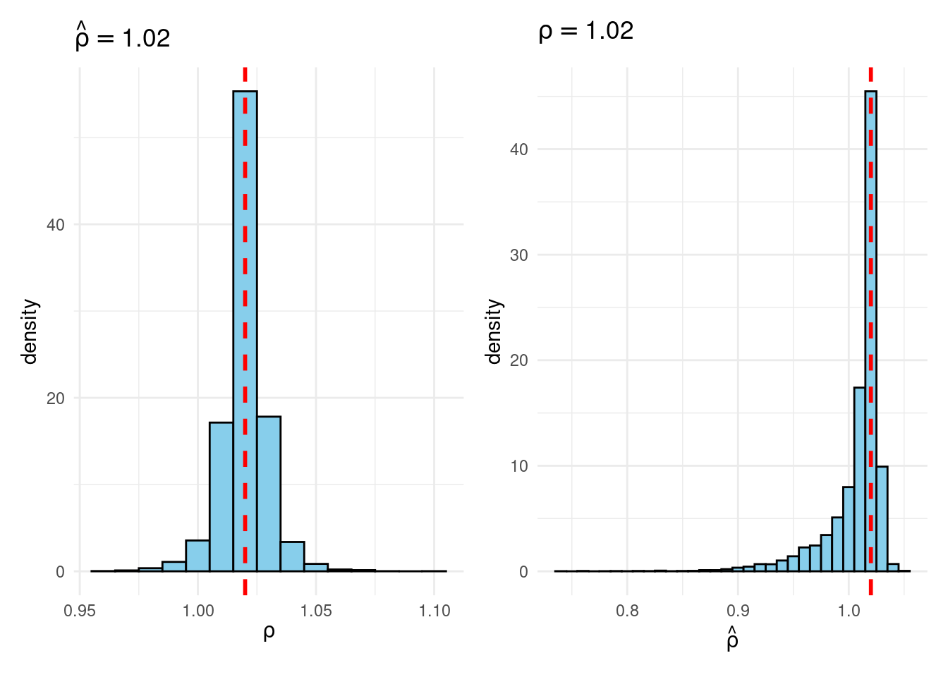
Their simulation contrasts the Frequentist sampling distribution of (widehat{rho}|rho) with the Bayesian posterior distribution of (rho|widehat{rho}) below a flat prior on (rho). When (rho) is close to one, these two distributions differ markedly: whereas the Bayesian posterior is all the time symmetric and centered at (widehat{rho} = widehat{rho}), the Frequentist sampling distribution is very skewed when (rho) is shut to 1. This exhibits that the Bayesian-Frequentist equivalence we present in our easy inhabitants imply instance from above breaks down fully on this extra advanced instance.

Sims & Uhlig argue that the Bayesian posterior gives a way more smart and helpful characterization of the knowledge contained within the knowledge and after studying the paper, I’m inclined to agree. My replication code follows under, together with plots of the joint distribution of ((rho, widehat{rho})) below a uniform prior for (rho) and the conditional distributions (widehat{rho}|rho=1) (Frequentist Sampling Distribution) and (rho|widehat{rho} = 1) (Bayesian Posterior).

The Replication

#-------------------------------------------------------------------------------
# Sims, C. A., & Uhlig, H. (1991). Understanding unit rooters: A helicopter tour
#
# (See additionally: Instance 6.10.6 from Poirier "Intermediate Statistics and 'Metrics")
#-------------------------------------------------------------------------------
# Within the subsequent part we are going to proceed to assemble, by Monte Carlo, an estimated
# joint pdf for rho and hat{rho} below a uniform prior pdf on rho. We select
# 31 values of rho, from 0.8 to 1.1 at intervals of 0.01. We draw 10000 100 x 1
# iid N(0,1) vectors of random variables to make use of a realizations of epsilon. For
# every of the 10000 epsilon vectors and every of the 31 rho values, we 
# assemble a y vector with y(0) = 0, y(t) generated by equation (1). 
#
# Equation (1): y(t) = rho y(t-1) + epsilon(t), t = 0, ..., T
#
# For every of those y vectors, we assemble hat{rho}. Utilizing as bins the
# intervals [-infty, 0.795), [0.795, 0.805), [0.805, 0.815), etc. we construct
# a histogram that estimates the pdf of hat{rho} for each fixed rho value. 
# When these histograms are lined up side by side, they form a surface that is
# the joint pdf for rho and hat{rho} under a flat prior on rho.
#-------------------------------------------------------------------------------
set.seed(1693)

library(tidyverse)
library(tictoc)
library(patchwork)

draw_rho_hat <- function(rho) {
# Carry out the simulation once for a fixed value of rho; return rho_hat
  nT <- 100
  y <- rep(0, nT + 1) 
  for (t in 2:(nT + 1)) {
    y[t] <- rho * y[t - 1] + rnorm(1)
  }
  y_t <- y[-1]
  y_tminus1 <- y[-length(y)]
  sum(y_t * y_tminus1) / sum(y_tminus1^2)
}

# Operate to run the simulation for a hard and fast worth of rho (10000 occasions)
run_sim <- (rho) map_dbl(1:1e4, (i) draw_rho_hat(rho))

tic()
foo <- run_sim(0.9)
toc() # ~0.6 seconds on my machine

## 0.595 sec elapsed

# Full sequence of rho values from Sims & Uhlig (1991)
rho <- seq(from = 0.8, to = 1.1, by = 0.01)

tic()
outcomes <- tibble(rho = rho, 
                  rho_hat = map(rho, run_sim)) # Listing columns
toc() # ~17 seconds on my machine (1991 was a very long time in the past!)

## 16.814 sec elapsed

# The outcomes tibble makes use of a listing column for rho_hat. That is handy for 
# making histograms of the frequentist sampling distribution (rho fastened) however
# not for making histograms of the Bayesian posterior (rho_hat) fastened. For the
# latter, we are going to use the unnest() perform to "develop" the checklist column rho_hat
# into a daily column. That is the "joint" distribution of rho and rho_hat.
joint <- outcomes |> 
  unnest(rho_hat)

joint |> 
  ggplot(aes(x = rho, y = rho_hat)) +
  geom_density2d_filled() + 
  coord_cartesian(ylim = c(0.8, 1.1)) + # Prohibit rho_hat axis
  labs(title = "Joint Distribution",
       x = expression(rho),
       y = expression(hat(rho))) +
  theme_minimal()

joint |> 
  filter(rho_hat >= 0.995 & rho_hat < 1.005) |>
  ggplot(aes(x = rho)) +
  geom_histogram(binwidth = 0.01, fill = "skyblue", coloration = "black") +
  labs(title = expression(hat(rho) == 1),
       x = expression(rho),
       y = "Frequency") +
  theme_minimal()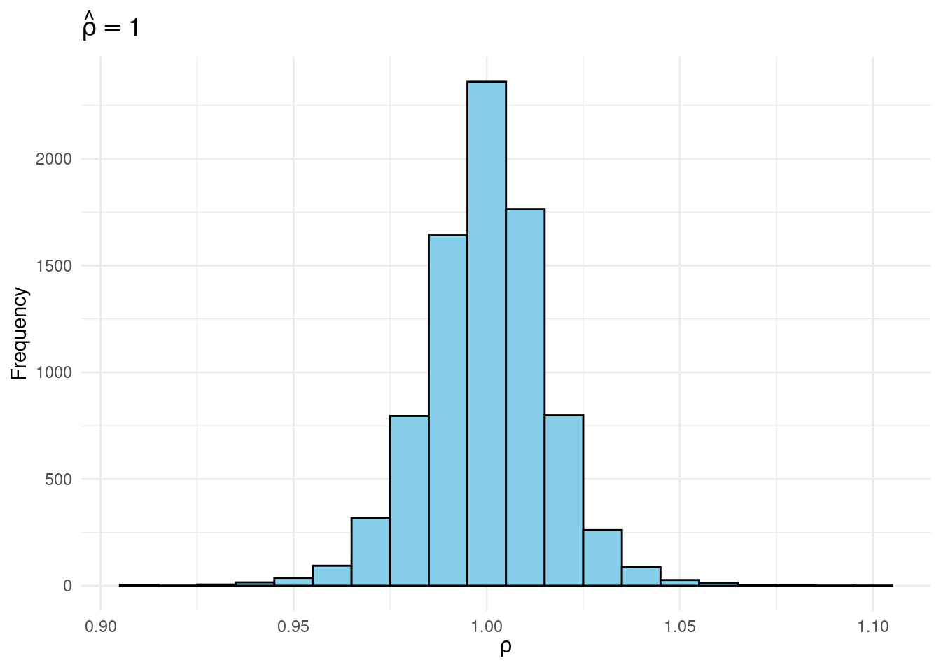

joint |> 
  filter(rho == 1) |> 
  ggplot(aes(x = rho_hat)) +
  geom_histogram(binwidth = 0.01, fill = "skyblue", coloration = "black") +
  labs(title = expression(rho == 1),
       x = expression(hat(rho)),
       y = "Frequency") +
  theme_minimal()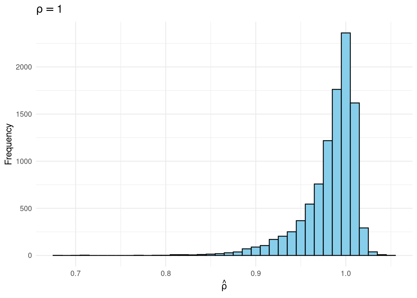

# Operate that makes the previous two plots, places them side-by-side and lets
# the person specify the worth of rho/rho_hat that we situation on:
plot_Bayes_vs_Freq <- (r) > 
    ggplot(aes(x = rho_hat)) +
    geom_histogram(aes(y = after_stat(density)), 
                   binwidth = 0.01, fill = "skyblue", coloration = "black") +
    geom_vline(xintercept = r, coloration = "purple", linetype = "dashed", linewidth = 1) +
    labs(title = bquote(rho == .(spherical(r, 3))),
         x = expression(hat(rho))) +
    theme_minimal()
  
  p1 + p2


plot_Bayes_vs_Freq(0.98)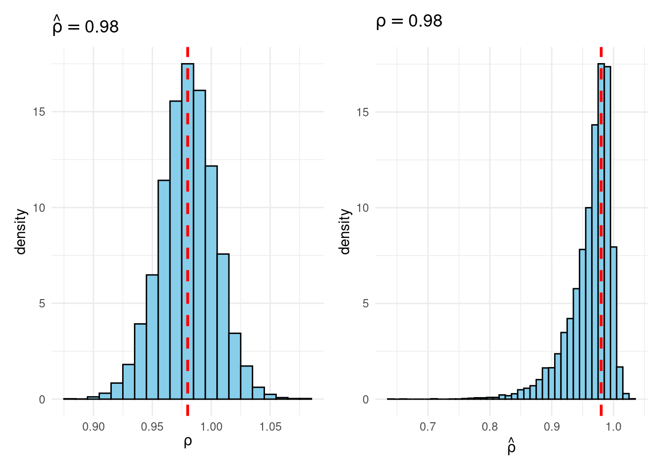

plot_Bayes_vs_Freq(0.99)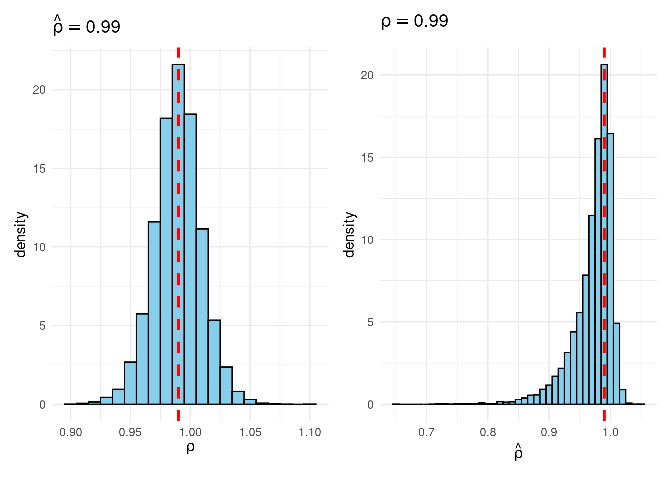

plot_Bayes_vs_Freq(1.0)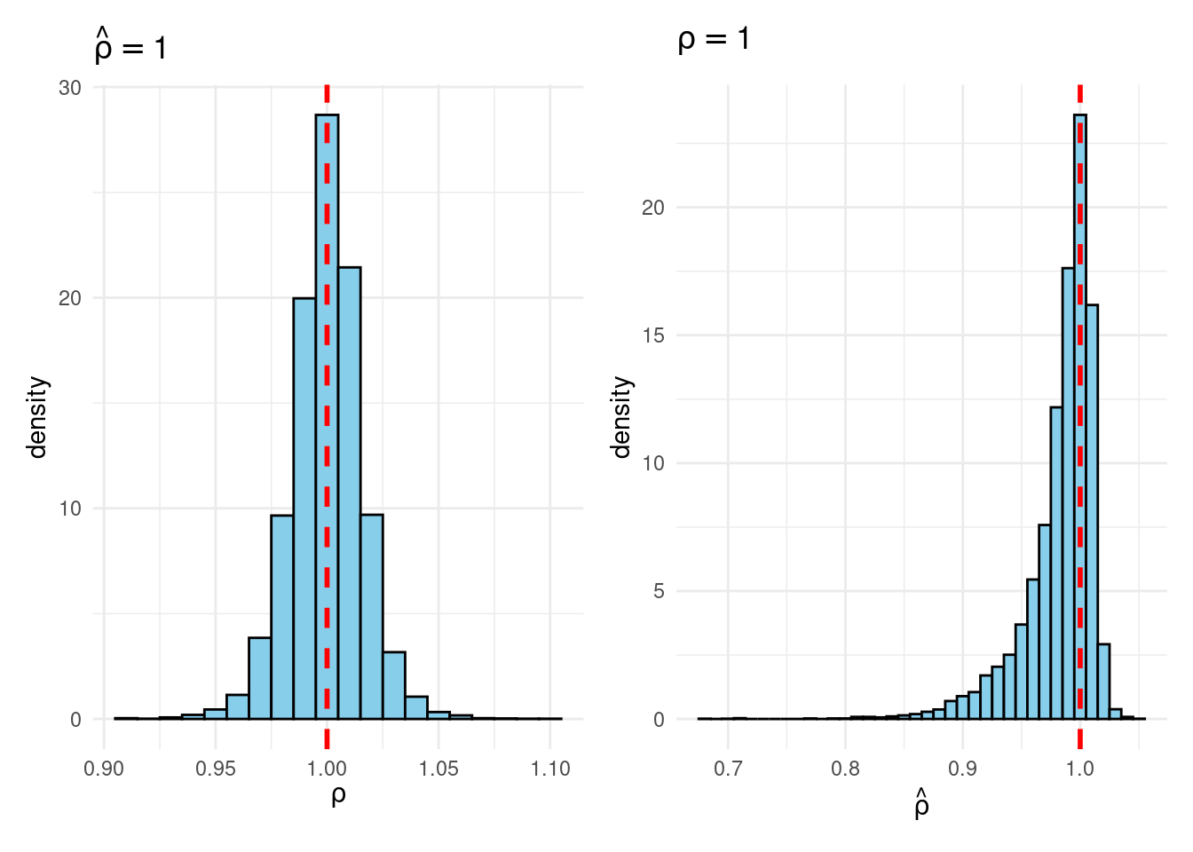

plot_Bayes_vs_Freq(1.01)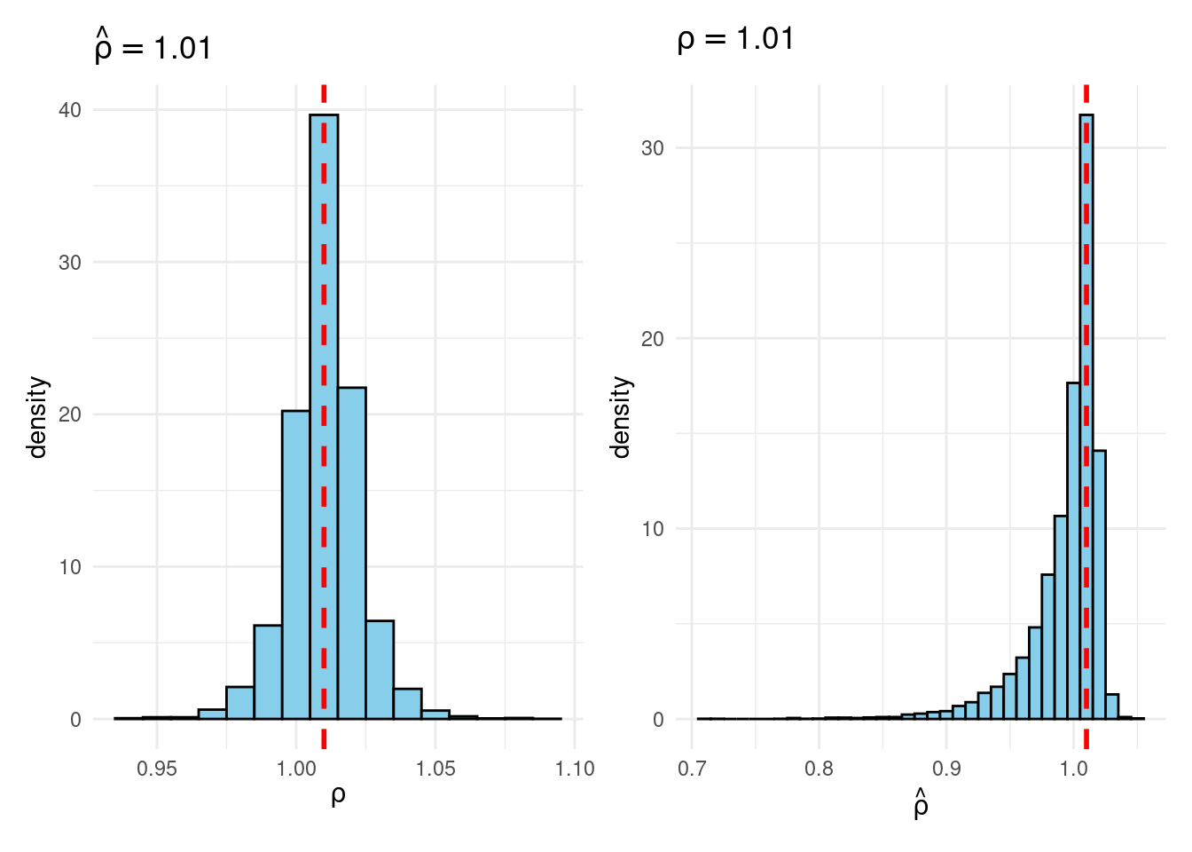

plot_Bayes_vs_Freq(1.02)