

I need to estimate, graph, and interpret the results of nonlinear fashions with interactions of steady and discrete variables. The outcomes I’m after will not be trivial, however acquiring what I would like utilizing margins, marginsplot, and factor-variable notation is simple.
Don’t create dummy variables, interplay phrases, or polynomials
Suppose I need to use probit to estimate the parameters of the connection
start{equation*}
P(y|x, d) = Phi left(beta_0 + beta_1x + beta_3d + beta_4xd + beta_2x^2 proper)
finish{equation*}
the place (y) is a binary end result, (d) is a discrete variable that takes on 4 values, (x) is a steady variable, and (P(y|x,d)) is the likelihood of my end result conditional on covariates. To suit this mannequin in Stata, I’d sort
probit y c.x##i.d c.x#c.x
I don’t must create variables for the polynomial or for the interactions between the continual variable (x) and the totally different ranges of (d). Stata understands that c.x#c.x is the sq. of (x) and that c.x##i.d corresponds to the variables (x) and (d) and their interplay. The results of what I typed would appear like this:
. probit y  c.x##i.d c.x#c.x

Iteration 0:   log chance = -686.40401
Iteration 1:   log chance = -643.73527
Iteration 2:   log chance = -643.44789
Iteration 3:   log chance = -643.44775
Iteration 4:   log chance = -643.44775

Probit regression                             Variety of obs     =      1,000
                                              LR chi2(8)        =      85.91
                                              Prob > chi2       =     0.0000
Log chance = -643.44775                   Pseudo R2         =     0.0626

----------------------------------------------------------------------------
           y |      Coef.   Std. Err.      z    P>|z|   [95% Conf. Interval]
-------------+--------------------------------------------------------------
           x |   .3265507   .0960978     3.40   0.001   .1382025    .5148988
             |
           d |
        uno  |   .3806342   .1041325     3.66   0.000   .1765382    .5847302
        dos  |   .5815309   .1177613     4.94   0.000    .350723    .8123388
       tres  |   .6864413   .1981289     3.46   0.001   .2981157    1.074767
             |
       d#c.x |
        uno  |  -.3163965   .1150582    -2.75   0.006  -.5419065   -.0908865
        dos  |  -.5075077   .1300397    -3.90   0.000  -.7623809   -.2526345
       tres  |  -.7081746   .2082792    -3.40   0.001  -1.116394   -.2999549
             |
     c.x#c.x |  -.1870304   .0339825    -5.50   0.000  -.2536349   -.1204259
             |
       _cons |  -.0357237   .0888168    -0.40   0.688  -.2098015    .1383541
----------------------------------------------------------------------------
I didn’t must create dummy variables, interplay phrases, or polynomials. As we are going to see under, comfort isn’t the one motive to make use of factor-variable notation. Issue-variable notation permits Stata to determine interactions and to differentiate between discrete and steady variables to acquire right marginal results.
This instance used probit, however most of Stata’s estimation instructions permit using issue variables.
Utilizing margins to acquire the results I’m occupied with
I’m occupied with modeling for people the likelihood of being married (married) as a operate of years of education (training), the percentile of revenue distribution to which they belong (percentile), the variety of instances they’ve been divorced (divorce), and whether or not their mother and father are divorced (pdivorce). I estimate the next results:
- The typical of the change within the likelihood of being married when every covariate adjustments. In different phrases, the typical marginal impact of every covariate.
- The typical of the change within the likelihood of being married when the interplay of divorce and training adjustments. In different phrases, a mean marginal impact of an interplay between a steady and a discrete variable.
- The typical of the change within the likelihood of being married when the interplay of divorce and pdivorce adjustments. In different phrases, a mean marginal impact of an interplay between two discrete variables.
- The typical of the change within the likelihood of being married when the interplay of percentile and training adjustments. In different phrases, a mean marginal impact of an interplay between two steady variables.
I match the mannequin:
probit married c.training##c.percentile c.training#i.divorce ///
    i.pdivorce##i.divorce
The typical of the change within the likelihood of being married when the degrees of the covariates change is given by
. margins, dydx(*)
Common marginal results Variety of obs = 5,000
Mannequin VCE : OIM
Expression : Pr(married), predict()
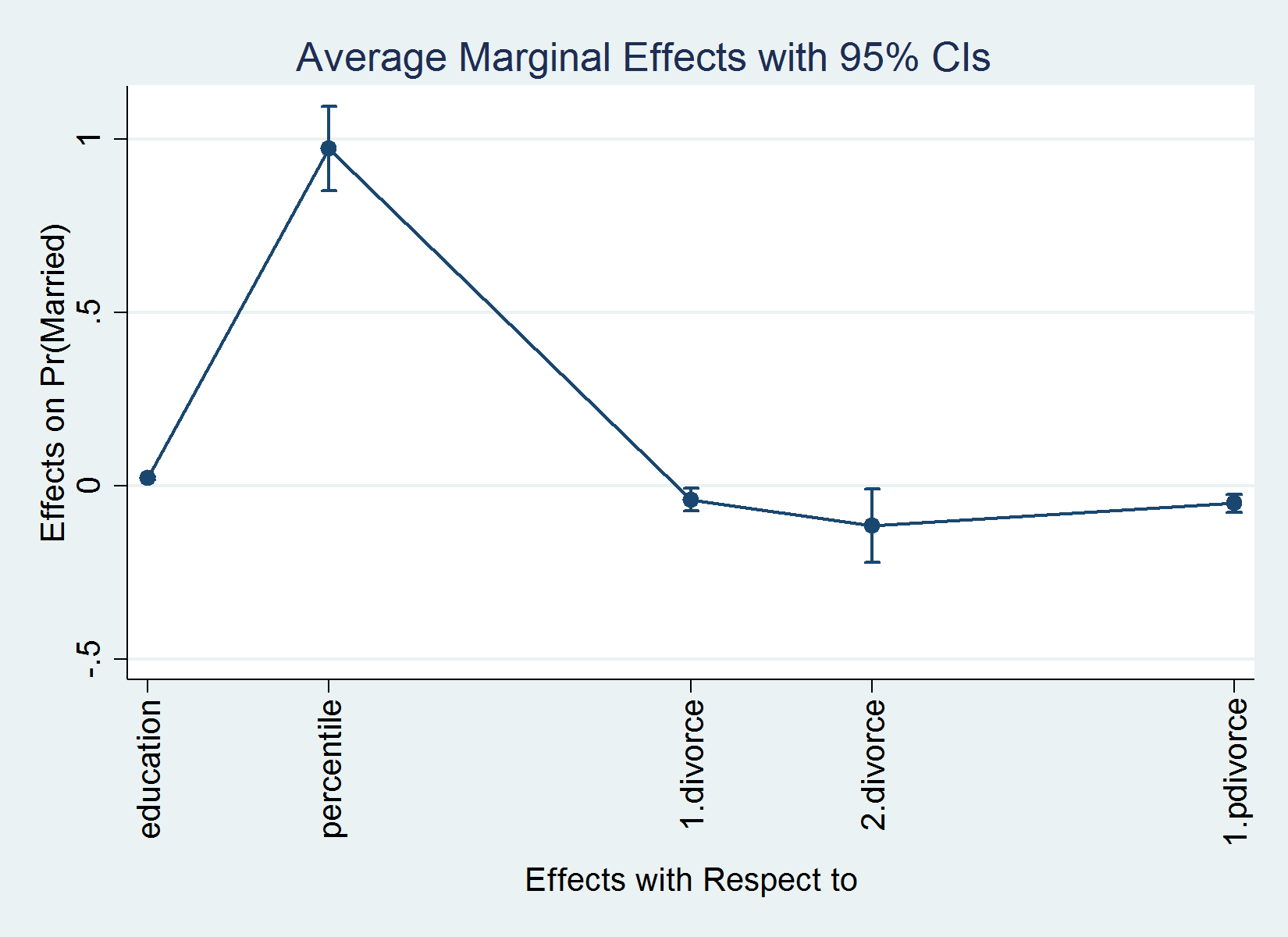
dy/dx w.r.t. : training percentile 1.divorce 2.divorce 1.pdivorce
----------------------------------------------------------------------------
| Delta-method
| dy/dx Std. Err. z P>|z| [95% Conf. Interval]
-------------+--------------------------------------------------------------
training | .02249 .0023495 9.57 0.000 .017885 .027095
percentile | .9873168 .062047 15.91 0.000 .8657069 1.108927
|
divorce |
1 | -.0434363 .0171552 -2.53 0.011 -.0770598 -.0098128
2 | -.1239932 .054847 -2.26 0.024 -.2314913 -.0164951
|
1.pdivorce | -.0525977 .0131892 -3.99 0.000 -.0784482 -.0267473
----------------------------------------------------------------------------
Observe: dy/dx for issue ranges is the discrete change from the bottom degree.
The primary a part of the margins output states the statistic it will compute, on this case, the typical marginal impact. Subsequent, we see the idea of an Expression. That is normally the default prediction (on this case, the conditional likelihood), however it may be every other prediction out there for the estimator or any operate of the coefficients, as we are going to see shortly.
When margins computes an impact, it distinguishes between steady and discrete variables. That is basic as a result of a marginal impact of a steady variable is a spinoff, whereas a marginal impact of a discrete variable is the change of the Expression evaluated at every worth of the discrete covariate relative to the Expression evaluated on the base or reference degree. This highlights the significance of utilizing factor-variable notation.
I now interpret a few the results. On common, a one-year change in training will increase the likelihood of being married by 0.022. On common, the likelihood of being married is 0.043 smaller within the case the place everybody has been divorced as soon as in contrast with the case the place nobody has ever been divorced, a mean therapy impact of (-)0.043. The typical therapy impact of being divorced two instances is (-)0.124.
Now I estimate the typical marginal impact of an interplay between a steady and a discrete variable. Interactions between steady and discrete variables are adjustments within the steady variable evaluated on the totally different values of the discrete covariate relative to the bottom degree. To acquire these results, I sort
. margins divorce, dydx(training) pwcompare

Pairwise comparisons of common marginal results
Mannequin VCE    : OIM

Expression   : Pr(married), predict()
dy/dx w.r.t. : training

--------------------------------------------------------------
             |   Distinction Delta-method         Unadjusted
             |      dy/dx   Std. Err.     [95% Conf. Interval]
-------------+------------------------------------------------
training    |
     divorce |
     1 vs 0  |   .0012968   .0061667     -.0107897    .0133833
     2 vs 0  |   .0403631   .0195432      .0020591    .0786672
     2 vs 1  |   .0390664   .0201597     -.0004458    .0785786
--------------------------------------------------------------
The typical marginal impact of training is 0.039 increased when everyone seems to be divorced two instances as an alternative of everybody being divorced one time. The typical marginal impact of training is 0.040 increased when everyone seems to be divorced two instances as an alternative of everybody being divorced zero instances. The typical marginal impact of training is 0 when everyone seems to be divorced one time as an alternative of everybody being divorced zero instances. One other approach of acquiring this result’s by computing a cross or double spinoff. As I discussed earlier than, we use derivatives for steady variables and variations with respect to the bottom degree for the discrete variables. I’ll consult with them loosely as derivatives hereafter. Within the appendix, I present that taking a double spinoff is equal to what I did above.
Analyzing the interplay between two discrete variables is just like analyzing the interplay between a discrete and a steady variable. We need to see the change from the bottom degree of a discrete variable for a change within the base degree of the opposite variable. We use the pwcompare and dydx() choices once more.
. margins pdivorce, dydx(divorce) pwcompare

Pairwise comparisons of common marginal results
Mannequin VCE    : OIM

Expression   : Pr(married), predict()
dy/dx w.r.t. : 1.divorce 2.divorce

--------------------------------------------------------------
             |   Distinction Delta-method         Unadjusted
             |      dy/dx   Std. Err.     [95% Conf. Interval]
-------------+------------------------------------------------
1.divorce    |
    pdivorce |
     1 vs 0  |  -.1610815   .0342655     -.2282407   -.0939223
-------------+------------------------------------------------
2.divorce    |
    pdivorce |
     1 vs 0  |  -.0201789   .1098784     -.2355367    .1951789
--------------------------------------------------------------
Observe: dy/dx for issue ranges is the discrete change from the
      base degree.
The typical change within the likelihood of being married when everyone seems to be as soon as divorced and everybody’s mother and father are divorced, in contrast with the case the place nobody’s mother and father are divorced and nobody is divorced, is a lower of 0.161. The typical change within the likelihood of being married when everyone seems to be twice divorced and everybody’s mother and father are divorced, in contrast with the case the place nobody’s mother and father are divorced and nobody is divorced, is 0. We might have obtained the identical consequence by typing margins divorce, dydx(pdivorce) pwcompare, which once more emphasizes the idea of a cross or double spinoff.
Now I have a look at the typical marginal impact of an interplay between two steady variables.
. margins,
>     expression(normalden(xb())*(_b[percentile] +
>     training*_b[c.education#c.percentile]))
>     dydx(training)

Common marginal results                      Variety of obs     =      5,000
Mannequin VCE    : OIM

Expression   : normalden(xb())*(_b[percentile] +
               training*_b[c.education#c.percentile])
dy/dx w.r.t. : training

----------------------------------------------------------------------------
             |            Delta-method
             |      dy/dx   Std. Err.      z    P>|z|   [95% Conf. Interval]
-------------+--------------------------------------------------------------
   training |   .0619111    .021641     2.86   0.004   .0194955    .1043267
----------------------------------------------------------------------------
The Expression is the spinoff of the conditional likelihood with respect to percentile. dydx(training) specifies that I need to estimate the spinoff of this Expression with respect to training. The typical marginal impact within the marginal impact of revenue percentile attributable to a change in training is 0.062.
As a result of margins can solely take first derivatives of expressions, I obtained a cross spinoff by making the expression a spinoff. Within the appendix, I present the equivalence between this technique and writing a cross spinoff. Additionally, I illustrate confirm that your expression for the primary spinoff is right.
Graphing
After margins, we are able to plot the leads to the output desk just by typing marginsplot. marginsplot works with the traditional graphics choices and the Graph Editor. For the primary instance above, as an illustration, I might sort
. quietly margins, dydx(*)

. marginsplot, xlabel(, angle(vertical))

  Variables that uniquely determine margins: _deriv
I added the choice xlabel(, angle(vertical)) to acquire vertical labels for the horizontal axis. The result’s as follows:
Conclusion
I illustrated compute, interpret, and graph marginal results for nonlinear fashions with interactions of discrete and steady variables. To interpret interplay results, I used the ideas of a cross or double spinoff and an Expression. I used simulated information and the probit mannequin for my examples. Nevertheless, what I wrote extends to different nonlinear fashions.
Appendix
To confirm that your expression for the primary spinoff is right, you evaluate it with the statistic computed by margins with the choice dydx(variable). For the instance within the textual content:
. margins,
>     expression(normalden(xb())*(_b[percentile] +
>     training*_b[c.education#c.percentile]))

Predictive margins                            Variety of obs     =      5,000
Mannequin VCE    : OIM

Expression   : normalden(xb())*(_b[percentile] +
               training*_b[c.education#c.percentile])

----------------------------------------------------------------------------
             |            Delta-method
             |     Margin   Std. Err.      z    P>|z|   [95% Conf. Interval]
-------------+--------------------------------------------------------------
       _cons |   .9873168    .062047    15.91   0.000   .8657069    1.108927
----------------------------------------------------------------------------

. margins, dydx(percentile)

Common marginal results                      Variety of obs     =      5,000
Mannequin VCE    : OIM

Expression   : Pr(married), predict()
dy/dx w.r.t. : percentile

----------------------------------------------------------------------------
             |            Delta-method
             |      dy/dx   Std. Err.      z    P>|z|   [95% Conf. Interval]
-------------+--------------------------------------------------------------
  percentile |   .9873168    .062047    15.91   0.000   .8657069    1.108927
----------------------------------------------------------------------------
Common marginal impact of an interplay between a steady and a discrete variable as a double spinoff:
. margins, expression(regular(_b[education]*training +
>          _b[percentile]*percentile +
>          _b[c.education#c.percentile]*training*percentile +
>          _b[1.divorce#c.education]*training +
>          _b[1.pdivorce]*pdivorce + _b[1.divorce] +
>          _b[1.pdivorce#1.divorce]*1.pdivorce +
>          _b[_cons]) -
>          regular(_b[education]*training +
>          _b[percentile]*percentile +
>          _b[c.education#c.percentile]*training*percentile
>          + _b[1.pdivorce]*pdivorce +
>          _b[_cons])) dydx(training)
Warning: expression() doesn't include predict() or xb().

Common marginal results                      Variety of obs     =      5,000
Mannequin VCE    : OIM

Expression   : regular(_b[education]*training + _b[percentile]*percentile +
               _b[c.education#c.percentile]*training*percentile +
               _b[1.divorce#c.education]*training + _b[1.pdivorce]*pdivorce
               + _b[1.divorce] + _b[1.pdivorce#1.divorce]*1.pdivorce +
               _b[_cons]) - regular(_b[education]*training +
               _b[percentile]*percentile +
               _b[c.education#c.percentile]*training*percentile +
               _b[1.pdivorce]*pdivorce + _b[_cons])
dy/dx w.r.t. : training

----------------------------------------------------------------------------
             |            Delta-method
             |      dy/dx   Std. Err.      z    P>|z|   [95% Conf. Interval]
-------------+--------------------------------------------------------------
   training |   .0012968   .0061667     0.21   0.833  -.0107897    .0133833
----------------------------------------------------------------------------
Common marginal impact of an interplay between two steady variables as a double spinoff:
. margins, expression(normalden(xb())*(-xb())*(_b[education]
>       + percentile*_b[c.education#c.percentile] +
>       1.divorce*_b[c.education#1.divorce] +
>       2.divorce*_b[c.education#2.divorce])*(_b[percentile] +
>       training*_b[c.education#c.percentile]) +
>       normalden(xb())*(_b[c.education#c.percentile]))

Predictive margins                            Variety of obs     =      5,000
Mannequin VCE    : OIM

Expression   : normalden(xb())*(-xb())*(_b[education] +
               percentile*_b[c.education#c.percentile] +
               1.divorce*_b[c.education#1.divorce] +
               2.divorce*_b[c.education#2.divorce])*(_b[percentile] +
               training*_b[c.education#c.percentile]) +
               normalden(xb())*(_b[c.education#c.percentile])

----------------------------------------------------------------------------
             |            Delta-method
             |     Margin   Std. Err.      z    P>|z|   [95% Conf. Interval]
-------------+--------------------------------------------------------------
       _cons |   .0619111    .021641     2.86   0.004   .0194955    .1043267
----------------------------------------------------------------------------
The simulated information:
clear
set obs 5000
set seed 111
generate training  = int(rbeta(4,2)*15)
generate percentile = int(rbeta(1,7)*100)/100
generate divorce    = int(rbeta(1,4)*3)
generate pdivorce   = runiform()<.6
generate e          = rnormal()
generate xbeta      = .35*(training*.06 + .5*percentile +   ///
                      .8*percentile*training                ///
                      + .07*training*divorce - .5*divorce - ///
                      .2*pdivorce - divorce*pdivorce - .1)
generate married    = xbeta + e > 0