

I wished to spotlight an intriguing paper I offered at a journal membership not too long ago:
There’s really a associated paper that got here out concurrently, learning full-batch gradient descent as a substitute of SGD:
Probably the most necessary insights in machine studying over the previous few years pertains to the significance of optimization algorithms in generalization efficiency.
Why deep studying works in any respect
To be able to perceive why deep studying works in addition to it does, it’s inadequate to cause in regards to the loss perform or the mannequin class, which is what classical generalisation concept focussed on. As a substitute, the algorithms we use to seek out minima (specifically, stochastic gradient descent) appear to play an necessary position. In lots of duties, highly effective neural networks are in a position to interpolate coaching knowledge, i.e. obtain near-0 coaching loss. There are the truth is a number of minima of the coaching loss that are just about indistinguishably good on the coaching knowledge. A few of these minima generalise properly (i.e. lead to low check error), others might be arbitrarily badly overfit.
What appears to be necessary then is just not whether or not the optimization algorithm converges rapidly to a neighborhood minimal, however which of the out there “just about world” minima it prefers to succeed in. It appears to be the case that the optimization algorithms we use to coach deep neural networks favor some minima over others, and that this choice leads to higher generalisation efficiency. The choice of optimization algorithms to converge to sure minima whereas avoiding others is described as implicit regularization.
I wrote this observe as an outline on how we/I at the moment take into consideration why deep networks generalize.
Analysing the impact of finite stepsize
One of many fascinating new theories that helped me think about what occurs in deep studying coaching is that of neural tangent kernels. On this framework we research neural community coaching within the restrict of infinitely vast layers, full-batch coaching and infinitesimally small studying charge, i.e. when gradient turns into steady gradient circulate, described by an odd differential equation. Though the speculation is beneficial and interesting, full-batch coaching with infinitesimally small studying charges could be very a lot a cartoon model of what we really do in apply. In apply, the smallest studying date does not at all times work greatest. Secondly, the stochasticity of gradient updates in minibatch-SGD appears to be of significance as properly.
What Smith et al (2021) do otherwise on this paper is that they attempt to research minibatch-SGD, for small, however not infinitesimally small, studying charges. That is a lot nearer to apply. The toolkit that permits them to review this situation is borrowed from the research of differential equations and known as backward error evaluation. The cartoon illustration under exhibits what backward error evaluation tries to realize:
For instance now we have a differential equation $dot{omega} = f(omega)$. The answer to this ODE with preliminary situation $omega_0$ is a steady trajectory $omega_t$, proven within the picture in black. We normally cannot compute this resolution in closed type, and as a substitute simulate the ODE utilizing the Euler’s methodology, $omega_{okay+1} = omega_k + epsilon f(omega_k)$. This leads to a discrete trajectory proven in teal. Because of discretization error, for finite stepsize $epsilon$, this discrete path might not lie precisely the place the continual black path lies. Errors accumulate over time, as proven on this illustration. The purpose of backward error evaluation is to discover a totally different ODE, $dot{omega} = tilde{f}(omega)$ such that the approximate discrete path we acquired from Euler’s methodology lieas close to the the continual path which solves this new ODE. Our purpose is to reverse engineer a modified $tilde{f}$ such that the discrete iteration might be well-modelled by an ODE.
Why is this convenient? As a result of the shape $tilde{f}$ takes can reveal fascinating features of the behaviour of the discrete algorithm, significantly if it has any implicit bias in the direction of shifting into totally different areas of the house. When the authors apply this system to (full-batch) gradient descent, it already suggests the form of implicit regularization bias gradient descent has.
In Gradient descent with a value perform $C$, the unique ODE is $f(omega) = -nabla C (omega)$. The modified ODE which corresponds to a finite stepsize $epsilon$ takes the shape $dot{omega} = -nablatilde{C}_{GD}(omega)$ the place
$$
tilde{C}_{GD}(omega) = C(omega) + frac{epsilon}{4} |nabla C(omega)|^2
$$
So, gradient descent with finite stepsize $epsilon$ is like operating gradient circulate, however with an added penalty that penalises the gradients of the loss perform. The second time period is what Barret and Dherin (2021) name implicit gradient regularization.
Stochastic Gradients
Analysing SGD on this framework is a little more tough as a result of the trajectory in stochastic gradient descent is, properly, stochastic. Subsequently, you do not have have a single discrete trajectory to optimize, however as a substitute you will have a distribution of various trajectories which you’d traverse for those who randomly reshuffle your knowledge. This is an image illustrating this example:
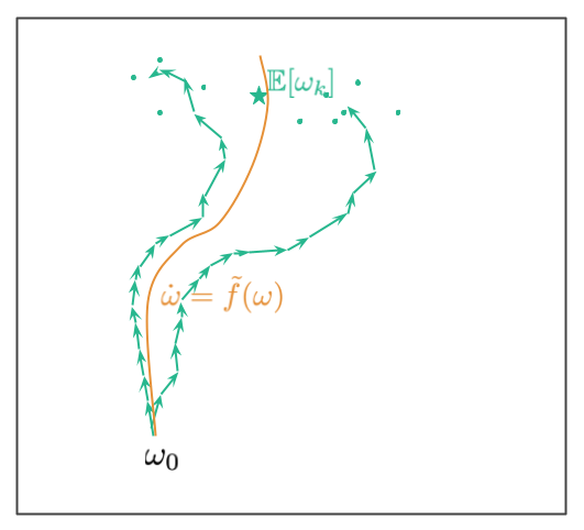
Ranging from the preliminary level $omega_0$ we now have a number of trajectories. These correspond to alternative ways we are able to shuffle knowledge (within the paper we assume now we have a hard and fast allocation of datapoints to minibatches, and the randomness comes from the order by which the minibatches are thought-about). The 2 teal trajectories illustrate two potential paths. The paths find yourself at a random location, the teal dots present further random endpoints the place trajectories might find yourself at. The teal star exhibits the imply of the distribution of random trajectory endpoints.
The purpose in (Smith et al, 2021) is to reverse-engineer an ODE in order that the continual (orange) path lies near this imply location. The corresponding ODE is of the shape $dot{omega} = -nabla C_{SGD}(omega)$, the place
$$
tilde{C}_{SGD}(omega) = C(omega) + frac{epsilon}{4m} sum_{okay=1}^{m} |nabla hat{C}_k(omega)|^2,
$$
the place $hat{C}_k$ is the loss perform on the $okay^{th}$ minibatch. There are $m$ minibatches in whole. Be aware that that is much like what we had for gradient descent, however as a substitute of the norm of the full-batch gradient we now have the typical norm of minibatch gradients because the implicit regularizer. One other fascinating view on that is to have a look at the distinction between the GD and SGD regularizers:
$$
tilde{C}_{SGD} = tilde{C}_{GD} + frac{epsilon}{4m} sum_{okay=1}^{m} |nabla hat{C}_k(omega) – C(omega)|^2
$$
This extra regularization time period, $frac{1}{m}sum_{okay=1}^{m} |nabla hat{C}_k(omega) – C(omega)|^2$, is one thing like the overall variance of minibatch gradients (the hint of the empirical Fisher data matrix). Intuitively, this regularizer time period will keep away from elements of the parameter-space the place the variance of gradients calculated over totally different minibatches is excessive.
Importantly, whereas $C_{GD}$ has the identical minima as $C$, that is not true for $C_{SGD}$. Some minima of $C$ the place the variance of gradients is excessive, is not a minimal of $C_{SGD}$. As an implication, not solely does SGD comply with totally different trajectories than full-batch GD, it could additionally converge to fully totally different options.
As a sidenote, there are various variations of SGD, primarily based on how knowledge is sampled for the gradient updates. Right here, it’s assumed that the datapoints are assigned to minibatches, however then the minibatches are randomly sampled. That is totally different from randomly sampling datapoints with alternative from the coaching knowledge (Li et al (2015) take into account that case), and certainly an evaluation of that variant might properly result in totally different outcomes.
Connection to generalization
Why would an implicit regularization impact avoiding excessive minibatch gradient variance be helpful for generalisation? Nicely, let’s take into account a cartoon illustration of two native minima under:
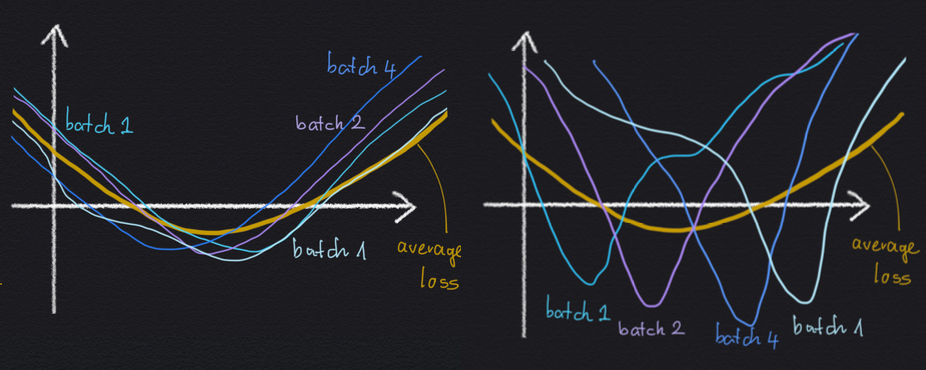
Each minima are the identical as a lot as the typical loss $C$ is anxious: the worth of the minimal is similar, and the width of the 2 minima are the identical. But, within the left-hand scenario, the vast minimal arises as the typical of a number of minibatch losses, which all look the identical, and which all are comparatively vast themselves. Within the right-hand minimal, the vast common loss minimal arises as the typical of quite a lot of sharp minibatch losses, which all disagree on the place precisely the situation of the minimal is.
If now we have these two choices, it’s cheap to count on the left-hand minimal to generalise higher, as a result of the loss perform appears to be much less delicate to whichever particular minibatch we’re evaluating it on. As a consequence, the loss perform additionally could also be much less delicate as to whether a datapoint is within the coaching set or within the check set.
Abstract
In abstract, this paper is a really fascinating evaluation of stochastic gradient descent. Whereas it has its limitations (which the authors do not attempt to disguise and focus on transparently within the paper), it nonetheless contributes a really fascinating new method for analysing optimization algorithms with finite stepsize. I discovered the paper to be well-written, with the reason of considerably tedious particulars of the evaluation clearly laid out. However maybe I favored this paper most as a result of it confirmed my intuitions about why SGD works, and what kind of minima it tends to favor.