

(defbfA{{bf A}}
defbfB{{bf }}
defbfC{{bf C}})Introduction
On this weblog put up, I describe Stata’s capabilities for estimating and analyzing vector autoregression (VAR) fashions with long-run restrictions by replicating among the outcomes of Blanchard and Quah (1989).
Framework
In earlier posts, I’ve recognized the parameters of a structural VAR mannequin by imposing restrictions on how shocks affect endogenous variables on affect. In contrast, Blanchard and Quah (1989) obtain identification by imposing restrictions on how shocks affect endogenous variables “in the long term”, that’s, the limiting response of an endogenous variable to a shock.
In a stationary VAR, the response of every variable to every shock should be zero within the restrict. Blanchard and Quah (1989) analyze a system composed of actual gross nationwide product (GNP) and unemployment, the place the expansion charge of GNP and the extent of the unemployment charge are assumed to be stationary. They’ve two shocks, which they time period “provide” and “demand” shocks, and the long-run response of GNP development and unemployment to these shocks should be zero as a result of these variables are stationary. The figuring out restriction is that an impulse to the “demand” shock has no impact on the extent of GNP in the long term. Therefore, the cumulative response of GNP development to the demand shock might be constrained to zero. The provision shock is thus outlined as that which ends up in a long-run change within the degree of GNP, and the demand shock is outlined as that which doesn’t change the long-run degree of GNP.
The Blanchard and Quah (1989) VAR is
start{align*}
bfA(L) start{bmatrix} Delta mathrm{gnp}_t mathrm{unrate}_t finish{bmatrix}
=
bfB start{bmatrix} e_t^{mathrm{provide}} e_t^{mathrm{demand}} finish{bmatrix}
finish{align*}
the place (L) is the lag operator and (bfA(L)) is a polynomial lag. We will invert the VAR into
start{align*}
start{bmatrix} Delta mathrm{gnp}_t mathrm{unrate}_t finish{bmatrix}
=
bfC(L) start{bmatrix} e_t^{mathrm{provide}} e_t^{mathrm{demand}} finish{bmatrix}
finish{align*}
The (bfC(L)) matrix is two-by-two and captures the long-run response to shocks. The identification assumption in Blanchard and Quah (1989) is that (C_{12}=0), which is equal to requiring that the extent of GNP ultimately return to 0 (or development) after a shock to the unemployment equation (the “demand” shock).
Information and replication
The information for this train are present in FRED codes GNPC96 and UNRATE, which I load into Stata utilizing the freduse command; see ssc set up freduse. The unemployment charge is measured because the quarterly common of month-to-month observations on UNRATE. GNP development is measured as 400 instances the log distinction in quarterly observations on GNP. Information within the Federal Reserve Financial Database are up to date over time due to the addition of recent observations and revisions to present observations, so the information I take advantage of won’t be similar to people who Blanchard and Quah (1989) used. The dataset I take advantage of will be downloaded right here.
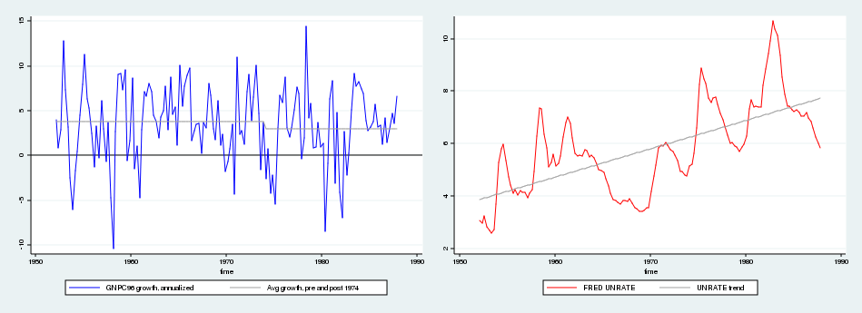
Blanchard and Quah (1989) use quarterly information from 1952 to 1987, which is proven under. The authors modify the uncooked information by eradicating the imply from GNP development individually for the pre-1974 and post-1974 subsamples and by eradicating a linear time development from the unemployment sequence.
After loading the uncooked information, I modify the unemployment and GNP development sequence in keeping with Blanchard and Quah’s (1989) article.
. use lrsvar.dta

. hold if 12 months >= 1952
(20 observations deleted)

. hold if 12 months <= 1987
(115 observations deleted)

. quietly regress unrate t

. predict unrate_adj, resid
The primary three traces load the information and limit the pattern to 1952–1987. The following two traces take away a time development from the unemployment sequence and retailer the residuals into unrate_adj.
Persevering with, I modify the GNP development sequence as in Blanchard and Quah (1989).
. generate bp1 = (12 months<1974)

. generate bp2 = (12 months>=1974)

. quietly regress development bp1 bp2, noconstant

. predict growth_adj, resid
The primary two traces create dummy variables, certainly one of which equals 1 earlier than the 1974 break level and the opposite of which equals 1 after the 1974 break level. The ultimate two traces take away the period-specific imply from GNP development and retailer the ensuing sequence into growth_adj.
The long-run structural VAR (SVAR) is estimated with svar utilizing the lreq() choice. Place GNP development first within the ordering. Then, the figuring out restriction is that the long-run GNP response to the unemployment shock is zero, which leads us to make use of the restriction matrix C = (.,0 .,.). On this matrix, three entries are free (set to lacking), and the remaining entry is compelled to zero. The authors use eight lags within the VAR, which I observe right here. We estimate the SVAR and create impulse–responses with
. matrix C = (., 0  .,.)

. svar growth_adj unrate_adj, lags(1/8) lreq(C)
Estimating long-run parameters

Iteration 0:   log probability = -1560.8311
Iteration 1:   log probability = -419.61266
Iteration 2:   log probability = -346.71202
Iteration 3:   log probability = -345.55296
Iteration 4:   log probability = -345.54985
Iteration 5:   log probability = -345.54985

Structural vector autoregression

 ( 1)  [c_1_2]_cons = 0

Pattern:  29 - 164                               Variety of obs     =        136
Precisely recognized mannequin                        Log probability    =  -345.5499

------------------------------------------------------------------------------
             |      Coef.   Std. Err.      z    P>|z|     [95% Conf. Interval]
-------------+----------------------------------------------------------------
      /c_1_1 |   1.512693   .0917205    16.49   0.000     1.332924    1.692462
      /c_2_1 |  -.3317345   .3803352    -0.87   0.383    -1.077178    .4137087
      /c_1_2 |          0  (constrained)
      /c_2_2 |   4.429225   .2685612    16.49   0.000     3.902855    4.955595
------------------------------------------------------------------------------

. irf create lr, set(lrirf) step(40) substitute
(file lrirf.irf now lively)
(file lrirf.irf up to date)
I’ve given the impulse–responses a reputation, lr, and saved them to a file, lrirf.irf.
We will view the impulse–responses with
. irf graph sirf, yline(0,lcolor(black)) xlabel(0(4)40) byopts(yrescale)
normal errors from all chosen outcomes are lacking, can't compute
    confidence intervals for the chosen statistics
The impulse–responses to every shock beneath the long-run identification scheme are held in sirf and are graphed within the subsequent determine. One step is one quarter, so the determine depicts the impulse–response over a interval of 10 years.
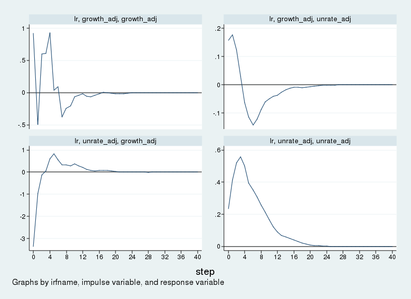
As a result of GNP development is ordered first, what Stata calls the “development impulse” is what Blanchard and Quah (1989) name the “provide” shock. Equally, the “unrate impulse” is the “demand” shock. The highest row reveals the response of GNP development and unemployment to a provide shock. GNP development rises; the unemployment charge rises on affect, then falls after about one 12 months, troughs after about two years, then slowly returns to its steady-state worth. The underside row reveals the response to a “demand” shock. In response to a “demand” shock, output development falls initially earlier than recovering after one 12 months. Unemployment rises, peaking a few 12 months after the shock earlier than returning to its steady-state worth.
Modifying the IRF graph
The impulse–responses within the above determine are when it comes to the expansion charge of GNP and the extent of the unemployment charge, as specified within the SVAR. It’s common as a substitute to graph the response of the extent of GNP. This entails creating an impulse–response graph that cumulates the response of GNP development however leaves the response of unemployment unchanged. This part seems to be contained in the .irf file and creates a sequence that accommodates the response of the extent of GNP and the extent of unemployment to shocks. Graphing the response of the extent of GNP can even extra clearly present the identification assumption we’ve made.
An .irf file is only a Stata information file with a selected nested panel construction. You possibly can entry it with use identical to some other dataset, and you’ll modify it identical to some other dataset.
The next code block creates a brand new variable, csirf, that holds the cumulative impulse–response of GNP development to every shock and does nothing to the impulse–response to the unemployment charge.
. use lrirf.irf, clear

. type irfname impulse response step

. gen csirf = sirf

. by irfname impulse: substitute csirf = sum(sirf) if response=="growth_adj"
(80 actual adjustments made)

. order irfname impulse response step sirf csirf

. save lrirf2.irf, substitute
file lrirf2.irf saved
The primary line imports the lrirf.irf dataset into Stata. The second line ensures that the information are sorted within the right order: first by irfname, then by the impulse variable, then by the response variable, and eventually by step. The third line generates our new variable, csirf, and hundreds it initially with the values in sirf. The fourth line replaces the values in csirf with the cumulation of values in sirf, however just for the response variable growth_adj, and does so by ifrname and impulse. I save the outcomes to a brand new irf file, lrirf2.irf. The result’s a variable that holds the cumulated response to adjustments in GNP development and leaves the responses to unemployment unchanged, which is what we sought.
We will graph the cumulated responses with
. irf set lrirf2.irf
(file lrirf2.irf now lively)

. irf graph csirf, yline(0,lcolor(black)) noci xlabel(0(4)40) byopts(yrescale)
and the accompanying graph is within the following determine.
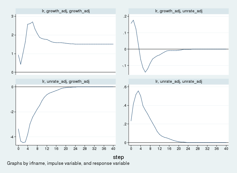
This determine will be in contrast with determine 1 in Blanchard and Quah (1989). The figures match apart from the size. Variations within the scale of the impulse–responses are as a consequence of variations within the measurement of the preliminary impulse. Stata makes use of a one-standard-deviation impulse, whereas Blanchard and Quah (1989) use a one-unit impulse. Within the top-left panel we see that the availability shock will increase the extent of GNP completely. Within the bottom-left panel, we see that GNP falls in response to a requirement shock however returns to zero (or development) over time. The long-run zero response within the bottom-left panel visually shows our identification assumption.
Conclusion
On this put up, I outlined a process to estimate a SVAR with long-run restrictions and confirmed how you can modify the ensuing IRF file to comprise a sequence that shows cumulative structural impulse–responses for some variables within the VAR.
Reference
Blanchard, O. J. and D. Quah. 1989. The dynamic results of combination demand and provide disturbances. American Financial Overview 79: 655–673.