

On this weblog submit, I’d like to present you a comparatively nontechnical introduction to Bayesian statistics. The Bayesian method to statistics has turn into more and more well-liked, and you may match Bayesian fashions utilizing the bayesmh command in Stata. This weblog entry will present a short introduction to the ideas and jargon of Bayesian statistics and the bayesmh syntax. In my subsequent submit, I’ll introduce the fundamentals of Markov chain Monte Carlo (MCMC) utilizing the Metropolis–Hastings algorithm.
Bayesian statistics by instance
Many people have been skilled utilizing a frequentist method to statistics the place parameters are handled as fastened however unknown portions. We will estimate these parameters utilizing samples from a inhabitants, however completely different samples give us completely different estimates. The distribution of those completely different estimates is named the sampling distribution, and it quantifies the uncertainty of our estimate. However the parameter itself continues to be thought-about fastened.
The Bayesian method is a distinct mind-set about statistics. Parameters are handled as random variables that may be described with chance distributions. We don’t even want information to explain the distribution of a parameter—chance is solely our diploma of perception.
Let’s work by way of a coin toss instance to develop our instinct. I’ll discuss with the 2 sides of the coin as “heads” and “tails”. If I toss the coin within the air, it should land on both the “heads” facet or the “tails” facet, and I’ll use (theta) to indicate the chance that the coin lands with the “heads” facet dealing with up.
Prior distributions
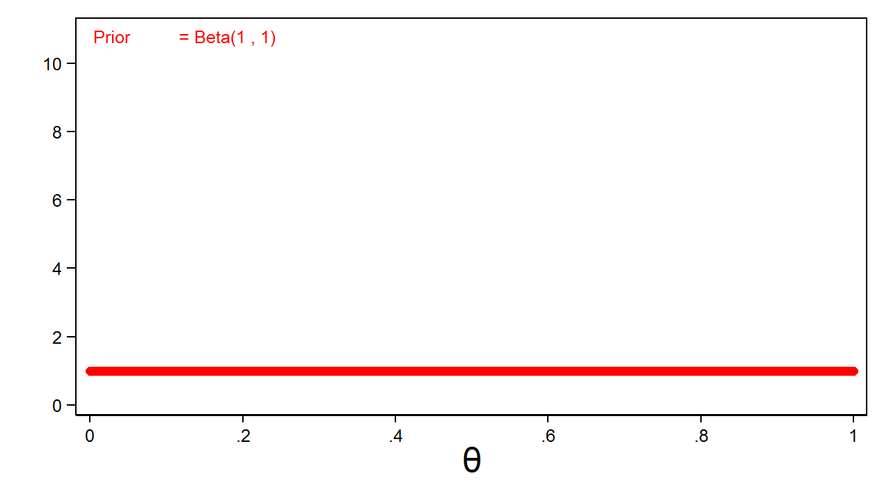
Step one in our Bayesian instance is to outline a previous distribution for (theta). A previous distribution is a mathematical expression of our perception in regards to the distribution of the parameter. The prior distribution might be based mostly on our expertise or assumptions in regards to the parameter, or it might be a easy guess. For instance, I might use a uniform distribution to specific my perception that the chance of “heads” might be wherever between zero and one with equal chance. Determine 1 reveals a beta distribution with parameters one and one that’s equal to a uniform distribution on the interval zero to 1.
Determine 1: Uninformative Beta(1,1) Prior
My beta(1,1) distribution is named an uninformative prior as a result of all values of the parameter have equal chance.
Frequent sense would recommend that the chance of heads is nearer to 0.5, and I might categorical this perception mathematically by rising the parameters of my beta distribution. Determine 2 reveals a beta distribution with parameters 30 and 30.
Determine 2: Informative Beta(30,30) Prior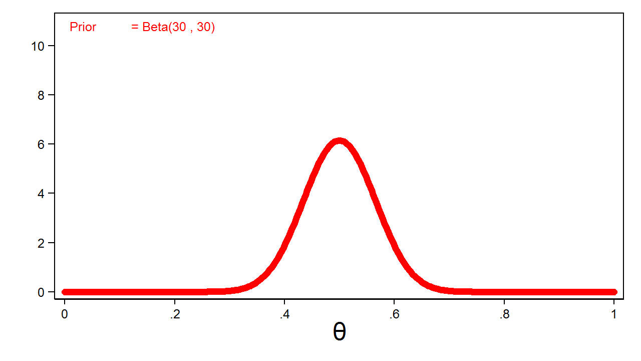
Determine 2 is named an informative prior as a result of all values of the parameter would not have equal chance.
Probability capabilities
The second step in our Bayesian instance is to gather information and outline a probability perform. Let’s say that I toss the coin 10 occasions and observe 4 heads. I then enter my leads to Stata in order that I can use the info later.
clear
enter heads
0
0
1
0
0
1
1
0
0
1
finish
Subsequent, I have to specify a probability perform for my information. Chance distributions quantify the chance of the info for a given parameter worth (that’s, (P(y|theta))), whereas a probability perform quantifies the probability of a parameter worth given the info (that’s, (L(theta|y))). The useful type is similar for each, and the notation is usually used interchangeably (that’s, (P(y|theta) = L(theta|y))).
The binomial chance distribution is usually used to quantify the chance of the variety of successes out of a hard and fast variety of trials. Right here I can quantify the outcomes of my experiment utilizing a binomial probability perform that quantifies the probability of (theta) given 4 heads out of 10 tosses.
The blue line in determine 4 reveals a binomial probability perform for theta given 4 heads out of 10 coin tosses. I’ve rescaled the graph of the probability perform in order that the realm below the curve equals one. This enables me to match the probability perform with the prior distribution graphed in crimson.
Determine 3: The Binomial(4,10,(boldsymbol{theta})) Probability Perform and the Beta(30,30) Prior Distribution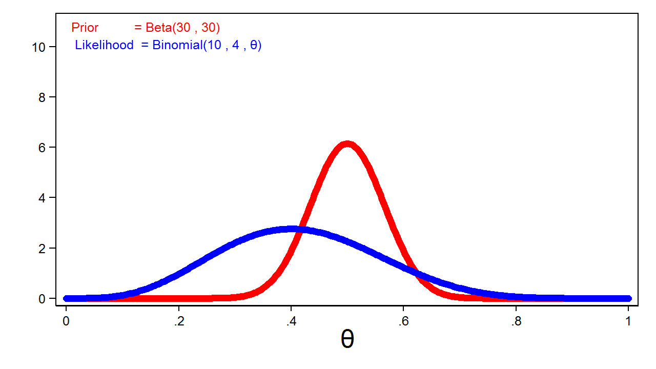
Posterior distributions
The third step in our Bayesian instance is to calculate a posterior distribution. This enables us to replace our perception in regards to the parameter with the outcomes of our experiment. In easy circumstances, we are able to compute a posterior distribution by multiplying the prior distribution and the probability perform. Technically, the posterior is proportional to the product of the prior and the probability, however let’s maintain issues easy for now.
[mathrm{Posterior} = mathrm{Prior}*mathrm{Likelihood}]
[P(theta|y) = P(theta)*P(y|theta)]
[P(theta|y) = mathrm{Beta}(alpha,beta)*mathrm{Binomial}(n,y,theta)]
[P(theta|y) = mathrm{Beta}(y+alpha,n-y+beta)]
On this instance, the beta distribution is named a “conjugate prior” for the binomial probability perform as a result of the posterior distribution belongs to the identical distribution household because the prior distribution. Each the prior and the posterior have beta distributions.
Determine 4 reveals the posterior distribution of theta with the prior distribution and the probability perform.
Determine 4: The Posterior Distribution, the Probability Perform, and the Prior Distribution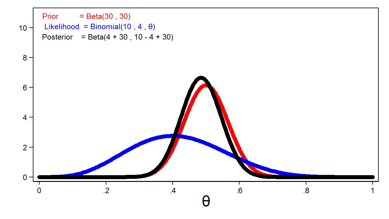
Discover that the posterior intently resembles the prior distribution. It is because we used an informative prior and a comparatively small pattern measurement.
Let’s discover the impact of various priors and pattern sizes on the posterior distribution. The crimson line in determine 5 reveals a very uninformative (mathrm{Beta}(1,1)) prior, and the probability perform is plotted in blue. You’ll be able to’t see the blue line as a result of it’s masked by the posterior distribution, which is plotted in black.
Determine 5: The Posterior Distribution For a Beta(1,1) Prior Distribution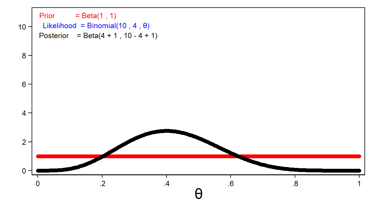
This is a crucial function of Bayesian evaluation: the posterior distribution will often be equal to the probability perform once we use fully uninformative priors.
Animation 1 reveals that extra informative priors could have higher affect on the posterior distribution for a given pattern measurement.
Animation 1: The impact of extra informative prior distributions on the posterior distribution
Animation 2 reveals that bigger pattern sizes will give the probability perform extra affect on the posterior distribution for a given prior distribution.
Animation 2: The impact of bigger pattern sizes on the posterior distribution
In apply, because of this we are able to scale back the usual deviation of the posterior distribution utilizing smaller pattern sizes once we use extra informative priors. However an identical discount in the usual deviation could require a bigger pattern measurement once we use a weak or uninformative prior.
After we calculate the posterior distribution, we are able to calculate the imply or median of the posterior distribution, a 95% equal tail credible interval, the chance that theta lies inside an interval, and plenty of different statistics.
Instance utilizing bayesmh
Let’s analyze our coin toss experiment utilizing Stata’s bayesmh command. Recall that I saved our information within the variable heads above. Within the bayesmh command in Instance 1, I’ll denote our parameter {theta}, specify a Bernoulli probability perform, and use an uninformative beta(1,1) prior distribution.
Instance 1: Utilizing bayesmh with a Beta(1,1) prior
. bayesmh heads, probability(dbernoulli({theta})) prior({theta}, beta(1,1))

Burn-in ...
Simulation ...

Mannequin abstract
------------------------------------------------------------------------------
Probability:
  heads ~ bernoulli({theta})

Prior:
  {theta} ~ beta(1,1)
------------------------------------------------------------------------------

Bayesian Bernoulli mannequin                         MCMC iterations  =     12,500
Random-walk Metropolis-Hastings sampling         Burn-in          =      2,500
                                                 MCMC pattern measurement =     10,000
                                                 Variety of obs    =         10
                                                 Acceptance charge  =      .4454
Log marginal probability = -7.7989401             Effectivity       =      .2391

------------------------------------------------------------------------------
             |                                                Equal-tailed
             |      Imply   Std. Dev.     MCSE     Median  [95% Cred. Interval]
-------------+----------------------------------------------------------------
       theta |  .4132299   .1370017   .002802   .4101121    .159595   .6818718
------------------------------------------------------------------------------
Let’s concentrate on the desk of coefficients and ignore the remainder of the output for now. We’ll talk about MCMC subsequent week. The output tells us that the imply of our posterior distribution is 0.41 and that the median can also be 0.41. The usual deviation of the posterior distribution is 0.14, and the 95% credible interval is [(0.16 – 0.68)]. We will interpret the credible interval the way in which we might usually wish to interpret confidence intervals: there’s a 95% probability that theta falls throughout the credible interval.
We will additionally calculate the chance that theta lies inside an arbitrary interval. For instance, we might use bayestest interval to calculate the chance that theta lies between 0.4 and 0.6.
Instance 2: Utilizing bayestest interval to calculate chances
. bayestest interval {theta}, decrease(0.4) higher(0.6)

Interval assessments     MCMC pattern measurement =    10,000

       prob1 : 0.4 < {theta} < 0.6

-----------------------------------------------
             |      Imply    Std. Dev.      MCSE
-------------+---------------------------------
       prob1 |     .4265     0.49459   .0094961
-----------------------------------------------
Our outcomes present that there’s a 43% probability that theta lies between 0.4 and 0.6.
Why use Bayesian statistics?
There are numerous interesting options of the Bayesian method to statistics. Maybe essentially the most interesting function is that the posterior distribution from a earlier examine can usually function the prior distribution for subsequent research. For instance, we would conduct a small pilot examine utilizing an uninformative prior distribution and use the posterior distribution from the pilot examine because the prior distribution for the primary examine. This method would improve the precision of the primary examine.
Abstract
On this submit, we centered on the ideas and jargon of Bayesian statistics and labored a easy instance utilizing Stata’s bayesmh command. Subsequent time, we are going to discover MCMC utilizing the Metropolis–Hastings algorithm.
You’ll be able to view a video of this matter on the Stata Youtube Channel right here:
Introduction to Bayesian Statistics, half 1: The essential ideas