

Introduction
Typically, I like to enhance a time-series graph with shading that signifies durations of recession. On this publish, I’ll present you a easy method so as to add recession shading to graphs utilizing knowledge offered by import fred. This publish additionally demostrates the right way to construct a posh graph in Stata, starting with the essential items and ending with a cultured product.
The Nationwide Bureau of Financial Analysis (NBER) defines a recession as “a major decline in financial exercise unfold throughout the economic system, lasting various months, usually seen in actual GDP, actual earnings, employment, industrial manufacturing, and wholesale–retail gross sales.” The NBER maintains a listing of turning-point months through which the “peaks” and “troughs” in enterprise exercise occurred. A recession is the time between a peak and a trough. As of February 2020, the checklist of recession dates is positioned at http://www.nber.org/cycles/cyclesmain.html.
The Federal Reserve Financial Database (FRED), maintained by the Federal Reserve Financial institution of St. Louis, comprises time-series knowledge on 1000’s of financial indicators from GDP and employment to change charges and commerce flows. It additionally comprises some utility sequence, one among which occurs to be an indicator variable that signifies whether or not a given month or quarter belongs to an NBER–outlined recession. We’ll use the import fred command to drag the FRED knowledge immediately into Stata.
Discovering and importing the information
I first add recession shading to a plot of the unemployment
fee. To import the information, I must know the FRED code for
the unemployment fee. I may look it up on-line, or I may search with
the FRED GUI, or I may search utilizing the fredsearch command.
More often than not, I might use the GUI, however for this publish I search
for it with fredsearch. The command takes a listing of key phrases as its
arguments, so typing
. fredsearch headline unemployment fee
searches for all sequence within the database that match all of the key phrases “headline”, “unemployment”, and “fee”. Extra key phrases will slender a search; fewer key phrases will choose up extra sequence.
. fredsearch headline unemployment fee
--------------------------------------------------------------------------------
Collection ID          Title                  Knowledge vary                Frequency
--------------------------------------------------------------------------------
CPIAUCSL           Shopper Worth Ind...  1947-01-01 to 2019-12-01  Month-to-month
UNRATE             Unemployment Price      1948-01-01 to 2020-01-01  Month-to-month
PAYEMS             All Staff, Tot...  1939-01-01 to 2020-01-01  Month-to-month
USSLIND            Main Index for ...  1982-01-01 to 2019-12-01  Month-to-month
CCSA               Continued Claims (...  1967-01-07 to 2020-01-25  Weekly, Endi
> ng Saturday
--------------------------------------------------------------------------------
Whole: 5
My search produced 5 outcomes. It appears to be like like UNRATE is the
meant goal. I verify this suspicion with one other fredsearch:
. fredsearch UNRATE, element
--------------------------------------------------------------------------------
UNRATE
--------------------------------------------------------------------------------
Title:                Unemployment Price
Supply:               U.S. Bureau of Labor Statistics
Launch:              Employment Scenario
Seasonal adjustment:  Seasonally Adjusted
Knowledge vary:           1948-01-01 to 2020-01-01
Frequency:            Month-to-month
Items:                %
Final up to date:         2020-02-07 07:47:02-06
Notes:                The unemployment fee represents the variety of unemploy...
--------------------------------------------------------------------------------
Whole: 1
The element choice offers extra element in regards to the matches discovered
by fredsearch.
Subsequent, I want the sequence that comprises the recession indicator. I carry out
one other fredsearch, this time trying to find nber recession.
. fredsearch nber recession, tags(usa month-to-month)
--------------------------------------------------------------------------------
Collection ID          Title                  Knowledge vary                Frequency
--------------------------------------------------------------------------------
USREC              NBER based mostly Recessi...  1854-12-01 to 2020-01-01  Month-to-month
USRECM             NBER based mostly Recessi...  1854-12-01 to 2020-01-01  Month-to-month
USRECP             NBER based mostly Recessi...  1854-12-01 to 2020-01-01  Month-to-month
USARECM            OECD based mostly Recessi...  1947-02-01 to 2019-12-01  Month-to-month
USAREC             OECD based mostly Recessi...  1947-02-01 to 2019-12-01  Month-to-month
USARECP            OECD based mostly Recessi...  1947-02-01 to 2019-12-01  Month-to-month
--------------------------------------------------------------------------------
Whole: 6
The tags() choice restricts the outcomes of the search to sequence
that match the tags. Considered use of key phrases and tags
narrows down the outcomes significantly. I exploit the usa tag to
prohibit my search to U.S. knowledge and the month-to-month tag to limit
my search to sequence with a month-to-month frequency. I selected a month-to-month
frequency as a result of the unemployment knowledge are reported month-to-month—see
the element output above. Three sequence appear like they could match: USREC, USRECM, and USRECP. I select USRECM as a result of, after a bit extra looking out, I discover that it’s the one which the St. Louis Fed makes use of.
I import the 2 sequence.
. import fred UNRATE USRECM

Abstract
--------------------------------------------------------------------------------
Collection ID                    Nobs    Date vary                Frequency
--------------------------------------------------------------------------------
UNRATE                       865     1948-01-01 to 2020-01-01  Month-to-month
USRECM                       1982    1854-12-01 to 2020-01-01  Month-to-month
--------------------------------------------------------------------------------
# of sequence imported: 2
   highest frequency: Month-to-month
    lowest frequency: Month-to-month
The import fred command imports every FRED code listed. It additionally offers two utility variables, datestr and daten. datestr is a string date variable, whereas daten is a numeric (day by day) date variable. The abstract desk offers details about every sequence: the identification code, the variety of observations, the date vary, and the statement frequency.
A graph with recession shading
Earlier than plotting, I must run some knowledge administration instructions.
First, I drop all observations for which the unemployment fee is
lacking. The recession indicator runs from 1854 to the current, whereas
the unemployment sequence runs solely from 1948 to the current. Second,
I generate just a few helpful time variables from the daten
variable. Third, I add concise labels to the unemployment fee and
recession variables.
. hold if UNRATE < .
(1,117 observations deleted)

. generate datem = mofd(daten)

. tsset datem, month-to-month
        time variable:  datem, 1948m1 to 2020m1
                delta:  1 month

. label variable UNRATE "Unemployment Price"

. label variable USRECM "Recession"
The generate datem = mofd(daten) command produces a Stata time
variable. The tsset command declares the information to be time-series knowledge. Lastly, the label variable command attaches labels to the variables.
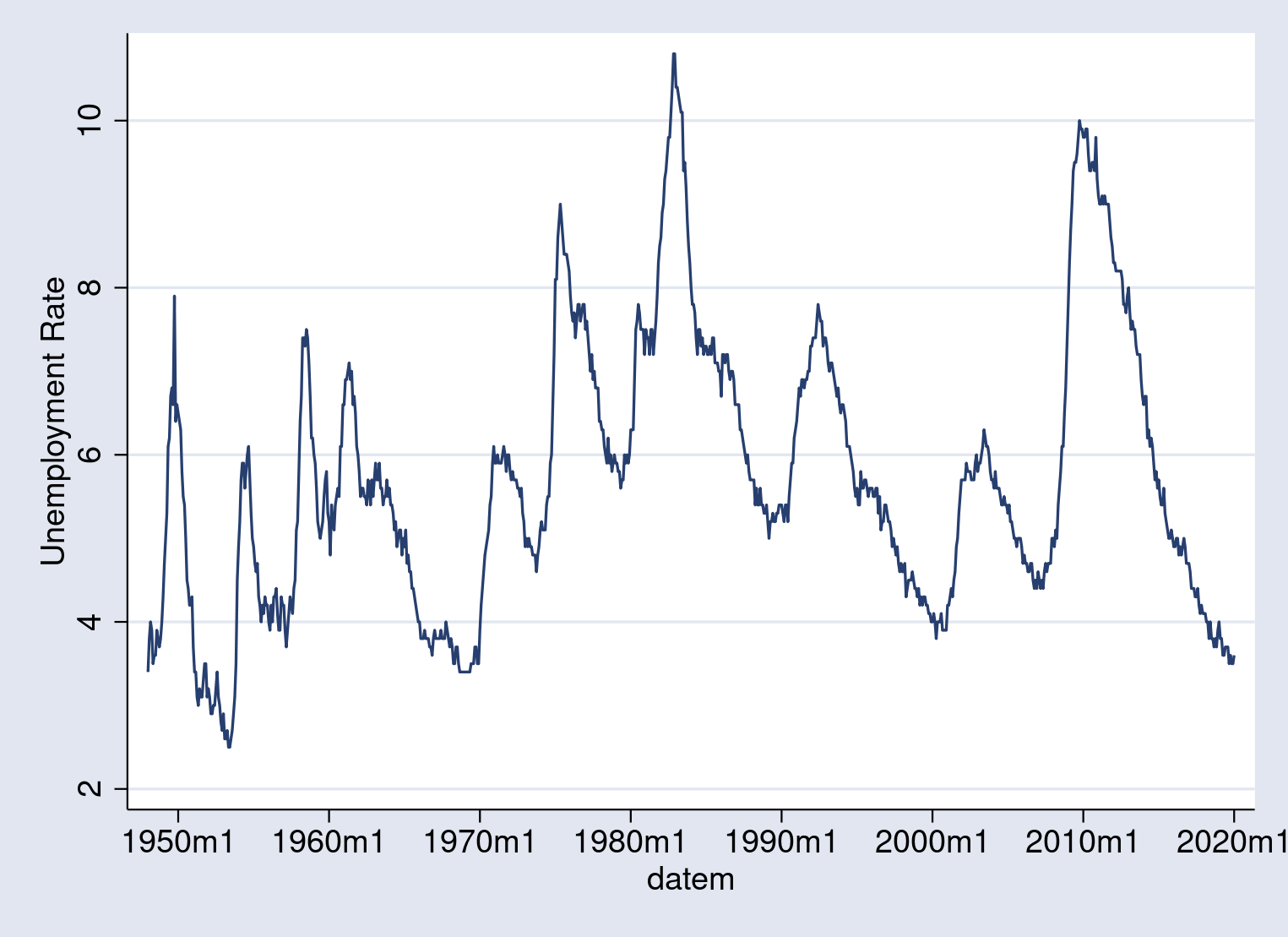
Let’s draw a preliminary graph of the unemployment fee with tsline:
. tsline UNRATE
This preliminary graph merely plots the unemployment fee with all default
graph choices. The information vary goes from about 3% to a little bit over 10%.
Subsequent, let’s draw a preliminary graph of the recession durations. The twoway space plot shades the world beneath a curve, so utilizing it on the recession indicator variable shades the recessions.
. twoway space USRECM datem
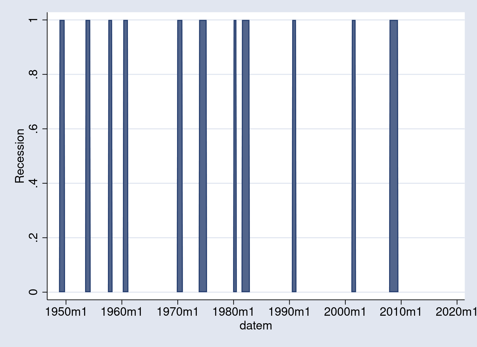
The indicator is 1 if the economic system is in recession throughout the month,
and 0 in any other case. From the earlier two graphs, the primary concept
turns into clear: so as to add recession shading to a graph, merely overlay the
unemployment fee plot on prime of the recession shading space plot.
We are able to mix the 2 graphs. However earlier than doing so, we have to stretch
the recession indicator in order that the peak of the recession bars covers the vary of the unemployment fee knowledge. As a result of the unemployment fee knowledge vary from 3 to about 10, I will stretch the recession indicator to equal 12 throughout a recession:
. exchange USRECM = 12*USRECM
(133 actual modifications made)
Multiplying the recession indicator by 12 transforms it from a
0–1 variable right into a 0–12 variable. Now, it’ll stretch
throughout the complete vary of unemployment charges.
Now, we are able to mix the plots utilizing twoway with every plot certain
by ().
. twoway (space USRECM datem) (tsline UNRATE)
The primary line is our space plot; the second line is our line plot.
Stata stacks the graphs from first to final, in order that the primary plot you
specify results in the background, whereas the final plot you specify ends
up within the foreground. The output appears to be like like this:
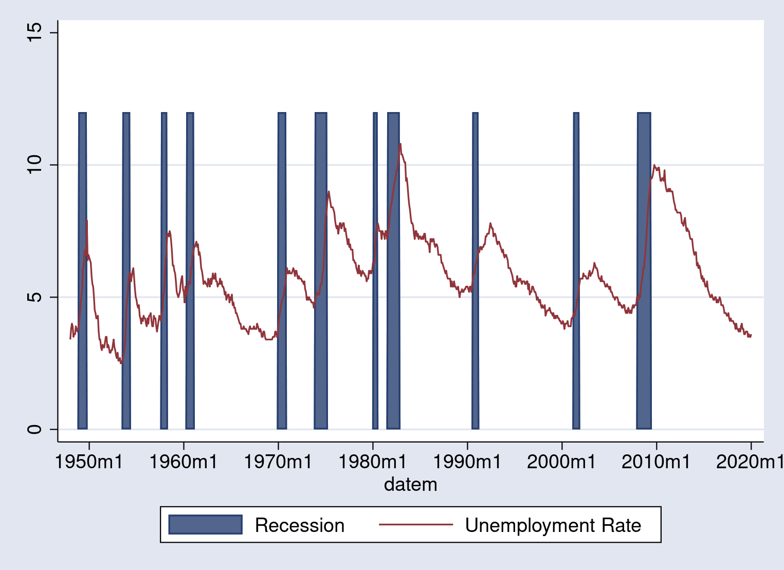
This graph exhibits off the concept, however the shading is just too darkish and the
axis labels want work. Luckily, graph twoway has a large suite of choices out there to switch the looks of the graph.
The final step is to make aesthetic changes to the graph to enhance
readability. We alter the scheme to pick our most well-liked general look, after which we modify particular person parts of the graph. We use choices inside twoway space to alter the colour of the shaded space; these particulars are modified by specifying the colour() choice. I select a light-gray shading, gs14. We use choices inside tsline to alter the looks of the unemployment fee plot; particularly, the road colour is managed by the lcolor() choice. I select a blue line. Choices specified outdoors the person plots will have an effect on all the graph. I alter the axis titles with xtitle() and ytitle() and alter the labels with tlabel() and ylabel(). When I’m finished, the command to run is
. set scheme s1color

. twoway  (space USRECM datem,   colour(gs14))
>         (tsline UNRATE,       lcolor(blue)),
>         ytitle("Unemployment fee")  xtitle("")
>         ylabel(0(3)12) tlabel(, format(%tmCCYY))
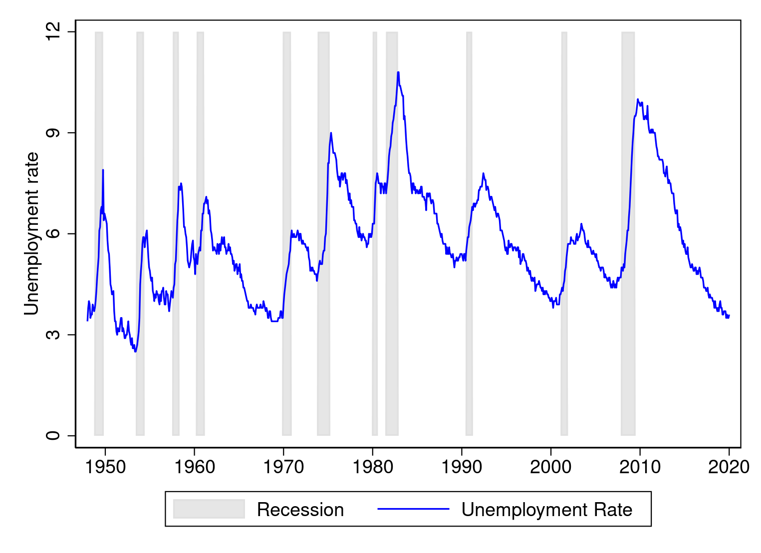
A lot better. Graphics instructions can get complicated. Stata has a “sort a little bit, get a little bit; sort so much, get so much” philosophy. The extra you sort, the extra management you’ve over the looks of the graph.
One other instance: Graphs with optimistic and detrimental values
As a second instance, I add recession shading to a graph of U.S. GDP
development. The FRED code for U.S. actual GDP development is A191RO1Q156NBEA.
GDP development knowledge are quarterly, so we use the quarterly recession indicator variable, which is USRECQM.
I import the information and carry out the mandatory cleanup.
. import fred A191RO1Q156NBEA USRECQM

Abstract
--------------------------------------------------------------------------------
Collection ID                    Nobs    Date vary                Frequency
--------------------------------------------------------------------------------
A191RO1Q156NBEA              288     1948-01-01 to 2019-10-01  Quarterly
USRECQM                      661     1854-10-01 to 2019-10-01  Quarterly
--------------------------------------------------------------------------------
# of sequence imported: 2
   highest frequency: Quarterly
    lowest frequency: Quarterly

. generate dateq   = qofd(daten)

. tsset dateq, quarterly
        time variable:  dateq, 1854q4 to 2019q4
                delta:  1 quarter
The import fred command imported the information, the generate dateq = qofd(daten) command generated a date variable, and the tsset command declared the information to be time-series knowledge.
The default identify of the GDP development variable is cumbersome, so I rename
it. I additionally give the sequence a pleasant label and drop any lacking observations.
. rename A191RO1Q156NBEA development

. label variable development "actual GDP development"

. hold if development < .
(373 observations deleted)
The following factor is to set the bounds of the recession shade space. Within the
earlier part, we summarized the unemployment fee and set the bounds
manually. This time, I summarize the development variable and use a few of the summarize command’s returned outcomes to set the bounds routinely. I create a brand new variable, recession, that holds a price equal to the utmost development fee when USRECQM equals one and holds the minimal development fee when USRECMQ equals zero. Therefore, the world shaded will vary vertically from the minimal to the utmost noticed GDP development fee.
. summarize development

    Variable |        Obs        Imply    Std. Dev.       Min        Max
-------------+---------------------------------------------------------
      development |        288    3.192361    2.565466       -3.9       13.4

. generate recession = r(max) if USREC == 1
(236 lacking values generated)

. exchange  recession = r(min) if USREC == 0
(236 actual modifications made)
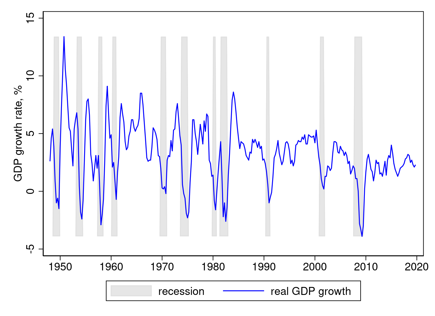
Let’s draw our graph with recession shading, following the identical
technique as earlier than:
. twoway  (space recession dateq,    colour(gs14))
>         (tsline development,           lcolor(blue)),
>         xtitle("") ytitle("GDP development fee, %")
The output is
That does not look proper. The habits of twoway space is to fill in
the world from the sting of the graph to the origin, which in our case means
that it fills from the highest down throughout recessions but in addition from the underside
up throughout expansions. The best way to repair it’s to make use of the base() choice
in twoway space.
The base() choice selects the worth to drop to. Let’s summarize development once more and this time retailer the worth of the minimal
in an area macro, min.
. summarize development

    Variable |        Obs        Imply    Std. Dev.       Min        Max
-------------+---------------------------------------------------------
      development |        288    3.192361    2.565466       -3.9       13.4

. native min = r(min)
We’ll use the worth saved in min when graphing. Alternatively,
we may have seemed on the output and manually copied the minimal
worth into the graph.
With the bottom worth in hand, let’s strive once more.
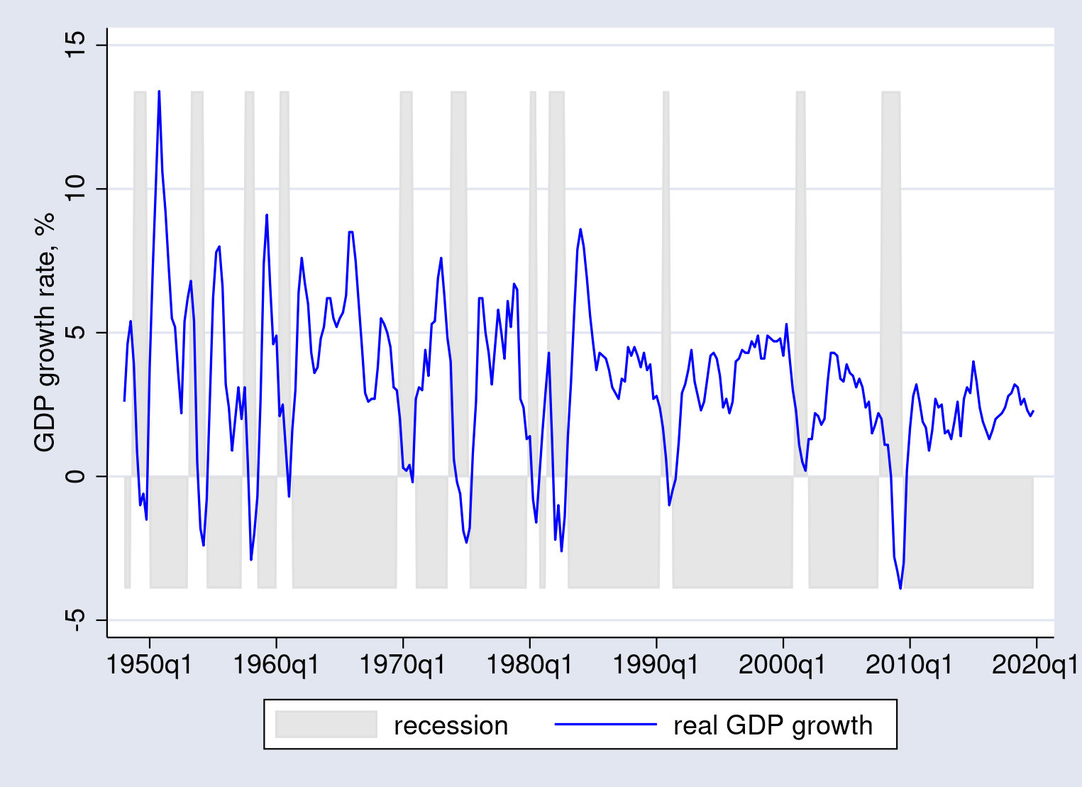
. set scheme s1color

. twoway  (space recession dateq,   colour(gs14)  base(`min'))
>         (tsline development,       lcolor(blue)),
>         xtitle("") ytitle("GDP development fee, %")
>         tlabel(, format(%tqCCYY))
Discover that I’ve specified the choice base(`min’) within the first
line, inside the space graph command. The output is
This appears to be like right. Substantively, recessions mark off durations of
lower-than-usual GDP development. Not all recessions are related
with detrimental GDP development; for instance, development slowed however didn’t flip detrimental throughout the 2001 recession. The recession of 2007–2009 is clearly seen, with deeply detrimental development
throughout 2008.
Conclusion
FRED offers a time-series marking U.S. recessions.
You possibly can import it as an indicator variable into Stata, then use that
indicator variable to attract recession shading in a time-series graph.
I demonstrated the right way to import sequence utilizing fredsearch and
import fred and the right way to construct an advanced graph out of less complicated
items.
Replication code
I walked you thru just a few instructions that didn’t work to point out
you when and why to make use of varied choices. The important instructions of the session had been
clear all

import fred UNRATE USRECM

hold if UNRATE < .
generate datem = mofd(daten)
tsset datem, month-to-month
label variable UNRATE "Unemployment Price"
label variable USRECM "Recession"

exchange USRECM = 12*USRECM

twoway (space USRECM datem, colour(gs14))               ///
       (tsline UNRATE,    lcolor(blue)),              ///
       xtitle("") ytitle("Unemployment fee")         ///
       ylabel(0(3)12) tlabel(, format(%tmCCYY))
clear all

import fred A191RO1Q156NBEA USRECQM
generate dateq = qofd(daten)
tsset dateq, quarterly

rename A191RO1Q156NBEA development
label variable development "actual GDP development"
hold if development < .

summarize development
generate recession = r(max) if USREC == 1
exchange recession  = r(min) if USREC == 0
native min = r(min)

set scheme s1color
twoway (space recession dateq, colour(gs14) base(‘min’))   ///
       (tsline development,  lcolor(blue)),                   ///
       xtitle("") ytitle("GDP development fee, %")           ///
       tlabel(, format(%tqCCYY))