

Introduction
The Federal Reserve Financial Database (FRED), maintained by the Federal Reserve Financial institution of St. Louis, makes accessible lots of of 1000’s of time-series measuring financial and social outcomes. The brand new Stata 15 command import fred imports knowledge from this repository.
On this publish, I present easy methods to use import fred to import knowledge from FRED. I additionally focus on a number of the metadata that import fred supplies that may be helpful in knowledge administration. I then exhibit easy methods to use a complicated characteristic: importing a number of revisions of sequence whose observations are up to date over time.
New knowledge releases replace practically all of the sequence in FRED. For some sequence, a brand new knowledge launch merely provides observations. For different sequence, a brand new knowledge launch can change the values of beforehand launched observations, as a result of the values of the observations are estimated or calculated. These adjustments are made as because the supply data adjustments or because the formulation or strategies change. For instance, the info on actual Gross Nationwide Product (GNP) in a selected quarter is up to date a number of instances as extra full supply data turns into accessible.
A revision of the info is called a classic. Vintages are recognized by the date of their launch; we communicate of “the July 10, 2017 classic”. The classic() possibility in import fred lets you entry earlier vintages of the info.
Prior vintages of knowledge have a number of makes use of. First, importing classic knowledge lets you view a dataset precisely as it might have been seen in an earlier paper, which is beneficial for replication functions. Second, prior vintages can be utilized as a robustness examine; in some contexts, it’s helpful to analyze whether or not your outcomes are sturdy throughout totally different vintages of the info. Third, in some utilized work, it’s essential to situation on data because it was accessible in actual time, moderately than use revised knowledge.
Within the instance mentioned beneath, later knowledge vintages reveal a deeper recession in 2008 than the sooner vintages.
Utilizing import fred
Like practically all instructions, you possibly can entry import fred by a menu-driven graphical person interface (GUI) and thru a command-line interface. The FRED repository is greatest explored utilizing the GUI accessible from the menu File > Import > Federal Reserve Financial Information (FRED). See [D] import fred, The FRED interface for an introduction to exploring FRED by way of the import fred GUI. Reproducible duties are simpler utilizing command-line interface. On this publish, I take advantage of the command-line interface as a result of functions of various vintages nearly at all times should reproducible.
Earlier than you possibly can reproduce what I do right here, you want a key to make use of FRED, which is freely accessible from
https://analysis.stlouisfed.org/docs/api/api_key.html
Click on on the hyperlink above, choose Request or view your API keys, then register to acquire a key. Then, in Stata, kind
. set fredkey key, completely
to set your key.
Collection in FRED are recognized by an alphanumeric code. FRED codes may be obscure; the import fred GUI and the fredsearch command can drastically assist to seek out the codes for the sequence you need. To search out the code for actual GNP, I take advantage of fredsearch. This command takes a listing of key phrases and searches for FRED sequence matching these key phrases. As well as, sequence in FRED have tags for nation, area, and many others., and fredsearch can limit the search to sequence matching these tags. Beneath, I take advantage of fredsearch to seek out the sequence with key phrases actual, gross, nationwide, and product. I add the choice tags(usa) to limit the search to U.S. knowledge sequence.
. fredsearch actual gross nationwide product, tags(usa)
--------------------------------------------------------------------------------
Collection ID          Title                  Information vary                Frequency
--------------------------------------------------------------------------------
GNPC96             Actual Gross Nationa...  1947-01-01 to 2017-01-01  Quarterly
GNPCA              Actual Gross Nationa...  1929-01-01 to 2016-01-01  Annual
Q0896AUSQ240SNBR   Gross Nationwide Professional...  1921-01-01 to 1939-10-01  Quarterly
A001RO1Q156NBEA    Actual Gross Nationa...  1948-01-01 to 2017-01-01  Quarterly
A791RX0Q048SBEA    Actual gross nationa...  1947-01-01 to 2017-01-01  Quarterly
A001RL1A225NBEA    Actual Gross Nationa...  1930-01-01 to 2016-01-01  Annual
A001RL1Q225SBEA    Actual Gross Nationa...  1947-04-01 to 2017-01-01  Quarterly
Q0896BUSQ008SNBR   Gross Nationwide Professional...  1947-01-01 to 1965-10-01  Quarterly
CB22RX1A020NBEA    Command-basis actual...  1929-01-01 to 2016-01-01  Annual
Q08321USQ008SNBR   Gross Nationwide Professional...  1947-01-01 to 1966-07-01  Quarterly
Q08328USQ350SNBR   Index of Labor Cos...  1948-01-01 to 1966-10-01  Quarterly
Q08300USQ259SNBR   Labor Value Per Dol...  1947-01-01 to 1966-07-01  Quarterly
B001RA3A086NBEA    Actual gross nationa...  1929-01-01 to 2016-01-01  Annual
CB22RX1Q020SBEA    Command-basis actual...  1947-01-01 to 2017-01-01  Quarterly
B001RA3Q086SBEA    Actual gross nationa...  1947-01-01 to 2017-01-01  Quarterly
--------------------------------------------------------------------------------
Whole: 15
The primary result’s the one we would like; the FRED code is GNPC96. I take advantage of import fred to import it.
. import fred GNPC96

Abstract
--------------------------------------------------------------------------------
Collection ID                    Nobs    Date vary                Frequency
--------------------------------------------------------------------------------
GNPC96                       281     1947-01-01 to 2017-01-01  Quarterly
--------------------------------------------------------------------------------
# of sequence imported: 1
   highest frequency: Quarterly
    lowest frequency: Quarterly
The abstract desk reviews the variety of sequence imported and the very best and lowest frequency of the imported sequence. The primary few observations are
. listing in 1/8, separator(4)

     +---------------------------------+
     | datestr          daten   GNPC96 |
     |---------------------------------|
  1. | 1947-01-01   01jan1947     1947 |
  2. | 1947-04-01   01apr1947   1945.3 |
  3. | 1947-07-01   01jul1947   1943.3 |
  4. | 1947-10-01   01oct1947   1974.3 |
     |---------------------------------|
  5. | 1948-01-01   01jan1948   2004.2 |
  6. | 1948-04-01   01apr1948   2037.2 |
  7. | 1948-07-01   01jul1948   2048.6 |
  8. | 1948-10-01   01oct1948   2050.8 |
     +---------------------------------+
datestr is a string variable containing the statement date. daten is the Stata each day date variable akin to the string date in datestr. By FRED conference, statement dates are saved as each day dates. For instance, the date for the primary quarter of 1947 is recorded as January 1, 1947.
We now use qofd() to create a quarterly date from daten, after which tsset the dataset:
. generate dateq = qofd(daten)

. tsset dateq, quarterly
        time variable:  dateq, 1947q1 to 2017q1
                delta:  1 quarter
import fred can import a number of sequence directly and may import sequence of various frequencies. It might probably combination high-frequency sequence right into a desired decrease frequency and may import knowledge over a requested date vary. For a full description of the capabilities of import fred, see http://www.stata.com/manuals/dimportfred.pdf.
Importing and inspecting vintages of a sequence
Having offered the important background materials, I now illustrate easy methods to import and plot a number of vintages of the GNPC96 sequence. Updates to this sequence are notably fascinating as a result of they reveal a decrease trough of the Nice Recession than these seen within the earlier knowledge releases.
We will import a number of vintages of actual GNP with a single import fred command by specifying the sequence’ FRED code and the specified vintages:
. import fred GNPC96, classic(2009-04-15 2010-04-15 2011-04-15 2017-04-15) clear

Abstract
--------------------------------------------------------------------------------
Collection ID                    Nobs    Date vary                Frequency
--------------------------------------------------------------------------------
GNPC96_20090415              248     1947-01-01 to 2008-10-01  Quarterly
GNPC96_20100415              252     1947-01-01 to 2009-10-01  Quarterly
GNPC96_20110415              256     1947-01-01 to 2010-10-01  Quarterly
GNPC96_20170415              280     1947-01-01 to 2016-10-01  Quarterly
--------------------------------------------------------------------------------
# of sequence imported: 4
   highest frequency: Quarterly
    lowest frequency: Quarterly
. generate dateq = qofd(daten)

. tsset dateq, quarterly
        time variable:  dateq, 1947q1 to 2016q4
                delta:  1 quarter
The primary command above imports 4 time sequence, one for every date specified. The title of every sequence consists of its FRED code and the date requested, so GNPC96_20090415 is the GNPC96 sequence as it might have been seen on April 15, 2009. The remaining instructions generate the quarterly variable and specify it because the tsset variable.
FRED sequence comprise metadata in regards to the sequence, together with the info supply, sequence title, frequency, items, and notes. import fred provides you entry to this metadata. Metadata about every imported sequence is saved within the variable traits. Traits are just like notes, however are primarily meant to be used in programming contexts. Within the case of import fred, the traits can comprise data that’s helpful in knowledge administration. Traits are considered with char listing and are referred to by varname[charname]. Two traits are of main curiosity when working with vintages. The attribute saved in Last_Updated comprises the classic date akin to the classic you imported.
. char listing GNPC96_20090415[Last_Updated]
  GNP~20090415[Last_Updated]: 2009-03-26 10:16:11-05

. char listing GNPC96_20100415[Last_Updated]
  GNP~20100415[Last_Updated]: 2010-03-26 13:31:07-05

. char listing GNPC96_20110415[Last_Updated]
  GNP~20110415[Last_Updated]: 2011-03-25 11:46:13-05

. char listing GNPC96_20170415[Last_Updated]
  GNP~20170415[Last_Updated]: 2017-03-30 08:01:04-05
The precise classic date related to GNPC96_20090415 is March 26, 2009. Once you specify a date that isn’t a real classic date, import fred imports the classic instantly previous to the date requested.
The attribute Items comprises the items that the sequence is measured in. This attribute is beneficial for sequence whose items could change over time. For instance, some sequence are adjusted for inflation and listed to a base yr; the bottom yr can change over time. Different sequence have items that don’t change over time. I listing the items for the 4 vintages I imported.
. char listing GNPC96_20090415[Units]
  GNP~20090415[Units]:        Billions of Chained 2000 {Dollars}

. char listing GNPC96_20100415[Units]
  GNP~20100415[Units]:        Billions of Chained 2005 {Dollars}

. char listing GNPC96_20110415[Units]
  GNP~20110415[Units]:        Billions of Chained 2005 {Dollars}

. char listing GNPC96_20170415[Units]
  GNP~20170415[Units]:        Billions of Chained 2009 {Dollars}
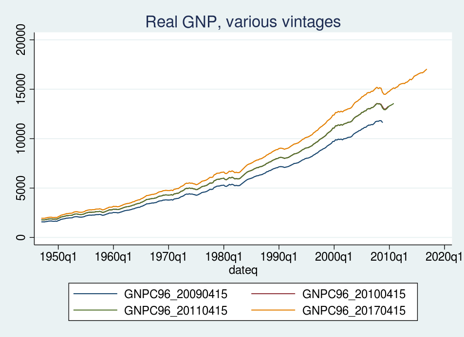
The items should not comparable throughout all vintages. One of many vintages makes use of a worth index measured in yr 2000 {dollars}; two others use yr 2005 {dollars}; and one makes use of yr 2009 {dollars}. The distinction in base yr seems as degree shifts in GNP. We will see these degree shifts by graphing the sequence:
. tsline GNPC96*, title("Actual GNP, varied vintages")
Revisions to the GNP progress charge
On this part, I illustrate that the revisions to GNP in these vintages yield surprisingly totally different progress charges. The subsequent few graphs plot actual GNP progress throughout the 2009, 2010, 2011, and 2017 vintages. GNP knowledge are sometimes reported in progress charges, and by utilizing progress charges we take away the extent shifts attributable to the change in base yr throughout vintages.
The expansion charge for every classic is calculated because the quarter-over-quarter share change in actual GNP. I label every classic with the yr of that classic.
. generate growth_2009 = 100*(GNPC96_20090415 / L.GNPC96_20090415 - 1)
(33 lacking values generated)

. label variable growth_2009 "2009"

. generate growth_2010 = 100*(GNPC96_20100415 / L.GNPC96_20100415 - 1)
(29 lacking values generated)

. label variable growth_2010 "2010"

. generate growth_2011 = 100*(GNPC96_20110415 / L.GNPC96_20110415 - 1)
(25 lacking values generated)

. label variable growth_2011 "2011"

. generate growth_2017 = 100*(GNPC96_20170415 / L.GNPC96_20170415 - 1)
(1 lacking worth generated)

. label variable growth_2017 "2017"
The lacking values for prior vintages happen as a result of, for instance, observations in 2015 don’t exist for the 2009 classic.
I subsequent graph the expansion charges calculated from every classic. First, I graph the 2009 and 2010 vintages collectively. After that, I graph all 4 vintages collectively.
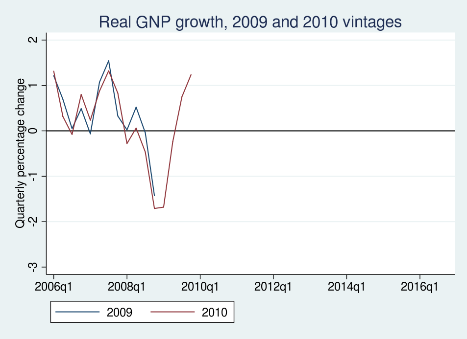
This graph plots the April 15, 2009 and April 15, 2010 vintages of actual GNP progress for every quarter ranging from the primary quarter of 2006. Items are in quarterly share change, so a price of two signifies 2% progress, quarter over quarter. A lot of the revisions are small and uninteresting, particularly in 2006 and 2007. Each vintages present that actual GNP progress slowed in 2008, however the 2010 classic signifies that progress slipped into destructive territory two quarters sooner than was estimated within the 2009 classic. Probably the most noticeable revisions are to the observations within the second and fourth quarters of 2008. The 2009 classic reviews that actual GNP fell by about 1.5% within the fourth quarter of 2008; the 2010 classic reviews a fall of 1.7%.
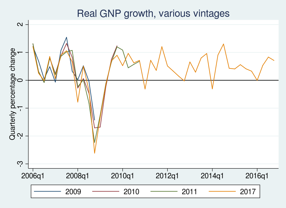
This graph provides the April 15, 2011 and April 15, 2017 vintages of actual GNP progress for every quarter ranging from the primary quarter of 2006. As earlier than, the revisions to observations in 2006 and 2007 are minor. The 2011 and 2017 vintages report a discount in GNP progress throughout 2008, relative to the 2009 classic. Most dramatic are the revisions to the statement in 2008q4. Whereas the 2009 classic reviews a decline in GNP progress of 1.5% in that quarter, the 2017 classic reviews a decline in GNP progress of practically 3%.
Conclusion
On this publish, I demonstrated easy methods to use import fred and easy methods to import a number of vintages of a sequence. I explored the revisions in actual GNP round 2008. Most revisions have been unremarkable, however the revisions in some quarters have been quantitatively giant and revealed a deeper recession trough than the sooner knowledge releases.