Imbens et al new undergrad course on causal inference in comparison with my very own, subsequent week’s diff-in-diff workshop and turning 50 (aka the second third)

I used to be happy the opposite day when I discovered that Guido Imbens and his colleague in pc science Mary Wooters, in addition to two graduate college students, Lea Bottmer and Jason Weitze, have since Fall 2024 developed a course on causal inference aimed toward freshmen and sophomores at Stanford. And I needed to point out it to you.

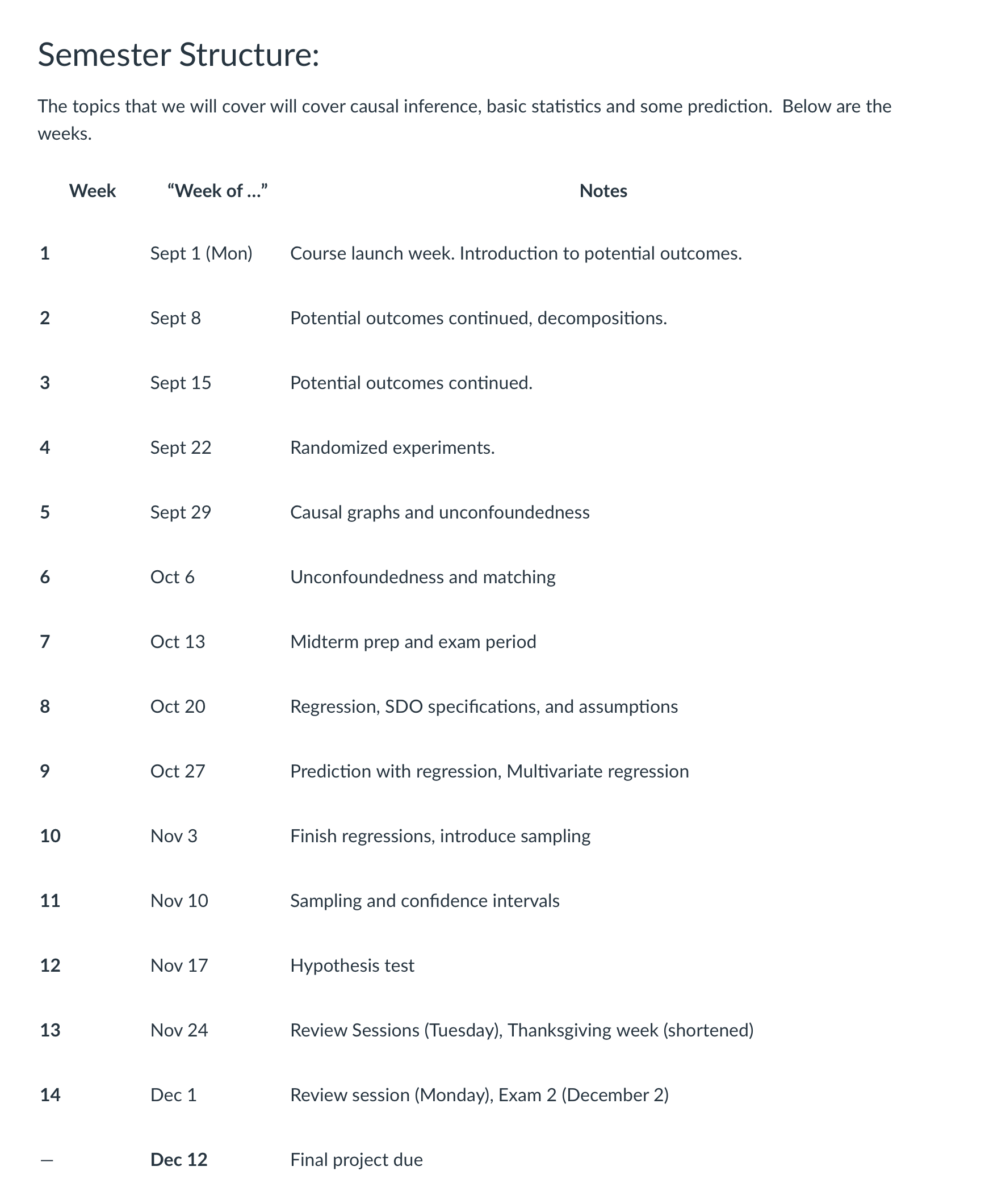
The course is titled “An Undergraduate Course in Causal Inference”. They wrote a paper simply accepted at Harvard Information Science Assessment which you will discover ungated model right here. And right here’s an image of the manager abstract of the course:

The category is for college kids that do not need a stats background. You will discover the supplies right here at their GitHub repo.

It was fascinating to learn Imbens, et al. class for a pair causes. First, I’ve been trying this too at Harvard within the Gov 50 class, “Quant Strategies for the Social Sciences”. My course define is right here.

I believe what I’ve seen is that my course gave the impression to be a little bit extra superior than theirs. Discover that I instantly lead instantly into potential outcomes. When you learn their paper, I don’t discover a lot about potential outcomes. You possibly can see for your self in case you and have a look at their first couple of lectures.

What they did instantly that I didn’t do was a “stats refresher” that emphasised imply, variance, commonplace errors, and confidence intervals. Whereas, I instantly went into level estimates solely. I truly don’t begin that till subsequent week, and it isn’t clear to me if that was sensible, however I’ll say it was intentional. I haven’t talked about “statistical significance” even as soon as this semester as a result of I felt that I actually needed to get them considering when it comes to populations solely. I frightened if I begins with a stats refresher, given they’d not any stats, that I couldn’t seize them. I had been taking the place this semester that:

So I used to be simply making an attempt to convey issues later. The one factor I actually labored with to date was the expectation operator which I tended to elucidate as “averages” however in school would usually say “weighted averages”.

The opposite factor I emphasised instantly was heterogenous remedy results. I did that as a result of I needed to show them the distinction between the typical remedy impact (ATE) and the typical remedy impact on the handled (ATT). And I did that as a result of a part of the aim of my course is:

1. use information in R

2. estimate fashions

3. appropriately interpret the numbers these fashions produce

4. inform the reality if you inform individuals about them

And you may get common remedy results however the portions be very totally different beneath heterogenous remedy results, however much more than that, I belong to the “parameters first” camp. Say the parameter, construct the mannequin, ask your self if beliefs assist that mannequin, then run the mannequin. And the mannequin specs for the ATE are totally different from the ATT. You see this significantly with regression which within the canonical additive mannequin:

doesn’t establish both the ATE or the ATT, however moderately a “bizarre weighted common” of the ATT and the ATU based mostly on variance weights that weight up the small teams and weight down the big teams. You must estimate a saturated regression adjustment model of that equation, do some algebra on the numbers it produces, after which you may get each the ATE and the ATT.

However, that was an excessive amount of for my class. What I opted to do as a substitute was simply emphasize up entrance the variations between all of them utilizing potential outcomes. I simply opted to guide instantly into potential outcomes as a result of I needed to see if my college students may do it. And to do this I created some worksheets that compelled them to calculate the decomposition of the easy distinction in imply outcomes into the ATE, choice bias and heterogenous remedy impact bias. That was how I then, too, introduced within the RCT, which Imbens, et al. additionally usher in early, as a result of beneath independence, the remedy and management group have:

1. the identical imply potential outcomes (together with counterfactuals)

2. the identical common remedy results (and thus ATT=ATU)

After which the easy distinction in imply outcomes recognized the ATE beneath randomized remedy task. The opposite factor that I’ve emphasised, however I doubt I pulled it off effectively, was the idea of the remedy task mechanism and its position in choice bias.

The opposite factor that’s totally different is I really feel like my slides are decidedly technical in comparison with what Imbens, et al. is doing. And I believe I simply must grow to be higher at making extra fascinating slides so it isn’t simply equations and phrases.

However all that stated, Imbens, et al. class actually appears proper to have “Lecture 0” introduce all the important thing concepts like unbiasedness, sampling, commonplace errors and confidence intervals. I didn’t convey it in till now, although, as a result of I made “easy comparisons” a central thought of my class, which I referred to as the SDO (“easy distinction in imply outcomes”). I needed individuals to see the SDO on a regular basis as a result of the decomposition we realized was expressed when it comes to the SDO on the left-hand-side, and if I made the SDO the central estimator, then I may hyperlink the RCT to bias. Plus there’s a easy regression specification that additionally estimates the SDO and that’s simply this:

And the delta-hat estimate from a regression was merely a distinction in two imply outcomes for when D=1 and D=0, respectively. And I did this as a result of I believed that if we simply may pin down that straightforward thought — and present the SDO each as a quantity and a visualization of two means as field plots the place variations of their two heights is the SDO — then it could allow me to maneuver into regression.

Which leads me to the second factor. I introduced in covariates beneath the technical time period “unconfoundedness”. It was difficult, to be trustworthy. Ideally I may’ve been extra profitable at serving to them construct fashions from scratch utilizing plug-in ideas implied by unconfoundedness, however as a substitute I simply went on to matching. I believed matching on Euclidean distance minimization the place the match was minimizing the sum of squared matching discrepancies might be the simpler thought than regression. And even earlier than that, I did actual matching, and regardless that imputation and reweightings are the identical factor, I believe to new individuals, reweighting the comparability teams is tougher to know than imputation, and I believe utilizing the closest neighbor matching used on Euclidean distance minimization was the simpler thought for all its flaws when assist breaks down. I additionally didn’t train the propensity rating as a result of the quantity of math I wanted to show probits was too excessive. However imputation is absolutely fairly easy — it makes use of variations, squaring, summing and sq. roots.

I simply felt like, additionally, if I used to be to give attention to level estimates, then it minimizes the quantity of issues that may journey them up — particularly arithmetic. The mathematics you want for potential outcomes based mostly causal parameters is averaging and variations. So in the event that they get confused, I informed them, it could possibly’t be due to the mathematics as a result of there’s nearly no math and what math is there’s trivial. So my thought was simply pen and paper and repetition via this decomposition worksheet.

And so the midterm lined potential outcomes, bias, mixture causal parameters (ATT, ATE, ATU), decompositions, RCT, unconfoundedness and matching, with a take residence that had them kind of copy a Lalonde script in direction of a unique dataset and interpret appropriately the numbers. That’s how I tended to speak too — “interpret the numbers appropriately”.

However, that stated, after the midterm I’ve been in regression as a result of regression like I stated makes easy comparisons when specified appropriately. After which I simply assumed fixed remedy results so I may skirt the problems about bizarre weights introduced up by Angrist 1999, after which later Tymon’s 2022 Restat. I simply felt like “bizarre regression weights” was not what I may pull off, so I didn’t. However because the regression coefficient in a bivariate regression is:

This was the place I might do two issues. First, I might train them learn how to manually calculate the intercept and regression coefficient utilizing very small datasets. I closely emphasised OLS minimizing the sum of squared residuals (which in case you squint, I’d already set them up for with nearest neighbor matching because it minimizes the sum of squared matching discreprancies which nearly really feel like residuals). I’m actually massive on creating worksheets, additionally. My feeling is that if they’ll’t do it with pencil and paper, it’s sufficiently advanced so to be magic. And I’m making an attempt to de-emphasize magic. So right here is the worksheet I gave them this week.

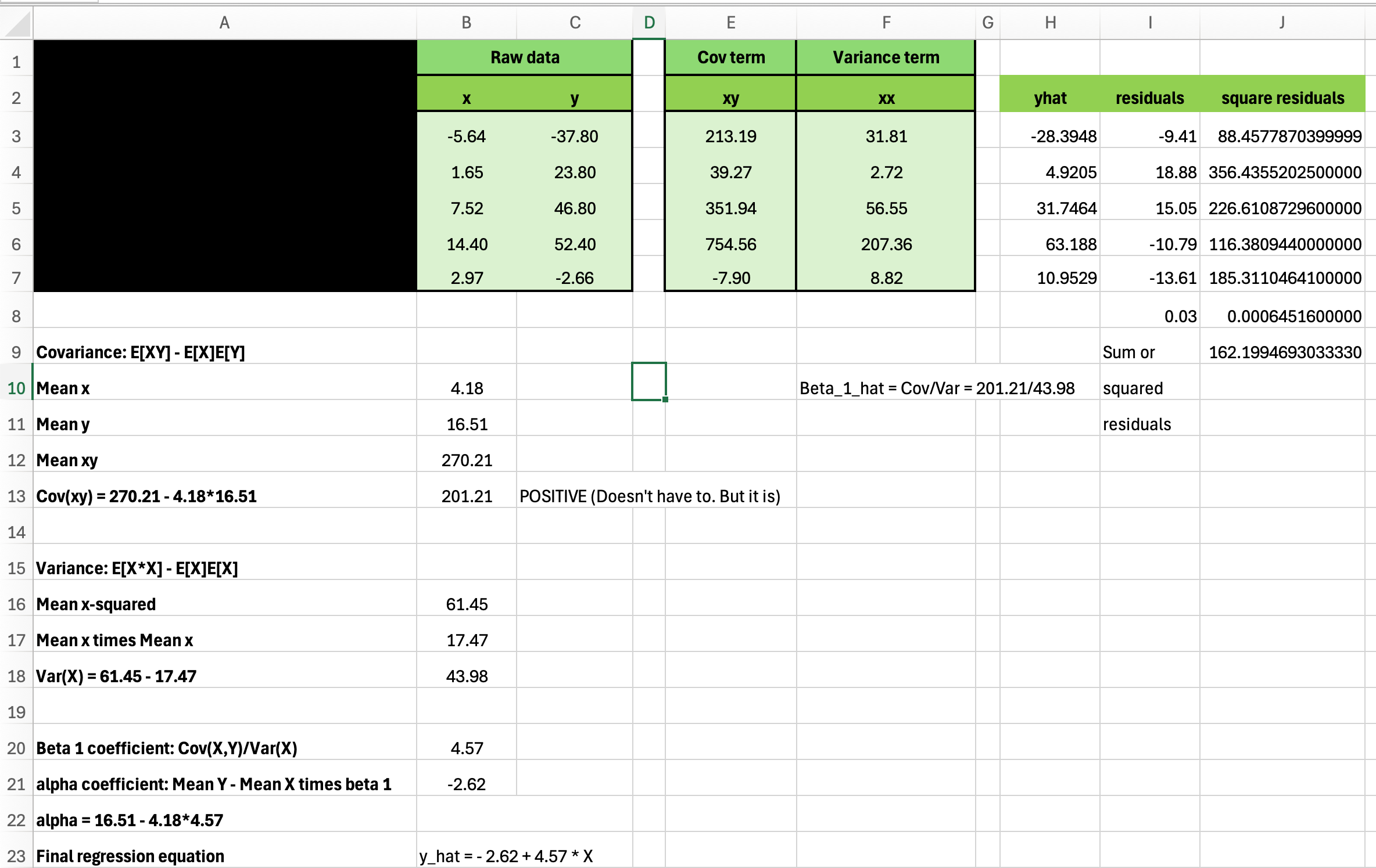
And see that is the place I launched covariance and variance. I gave them a “dataset” of 5 items (columns B and C), and confirmed them precisely the formulation for covariance, variance and the intercept and coefficient on the RHS covariate. This was an additional credit score task additionally price +2 factors on the following midterm, and it had be accompanied by an R quarto doc that estimated regression coefficients utilizing:

ols <- lm(y ~ x)
ols

After which examine that with calculating the regression coefficients from calculating covariance, variance and means for the intercept and coefficient equations. And the worksheet had 6 datasets. And the aim was easy:

1. By repetition, be taught the equations via muscle reminiscence

2. Use R as a calculator and do it once more

3. Begin studying variance

So, whereas Imbens, et al. launched variance on day 1, I don’t till now and particularly I did within the context of regression. I did this due to this previous pedagogical perception of mine based mostly on one thing I as soon as heard Jerry Seinfeld’s spouse say on this cookbook she wrote. She stated in it that the best way she received her children to eat their veggies was to place it on a pizza. And that’s how I considered variance — I’ll simply make regression one other estimator, make them calculate covariance and variance like 10 instances manually and utilizing R, after which slide into variance by making footage. Particularly this image:

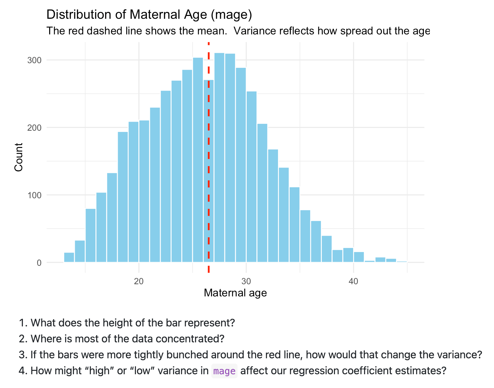
And this was the place I attempted to get them to consider variance — do it inside regression equations. The thought too was that since variance is within the denominator, they’d see you may’t estimate the coefficient on variable that may be a fixed because it’s variance is zero, and so it simply falls into the intercept.

The thought right here is I’ve been simply making an attempt to maneuver via steps however by making causal inference first and statistical inference second. My perspective has been that as long as the category concludes with all the pieces, the order during which they be taught it doesn’t matter. As long as they get from level A to level B, who’s to say which path is quicker, or if quicker even is crucial aim. All of us have one semester to get there and my approach tries to sneak the veggies on the pizza, moderately than take all of the substances, lay them out, and discuss them individually first.

Additionally I’m speaking about commonplace deviations inside variance by simply speaking about variance as having squared the items and thus turns into onerous to speak about. As an illustration, within the above image, I’ve plotted maternal age. And so the variance is “age-squared” which isn’t actually a pure approach of speaking. However since the usual deviation takes the sq. root of the variance, its items return to the unique type of “age”, and that’s straightforward to speak about. So then I’ve them do make utilizing ggplot the identical plot however with commonplace deviations proven:

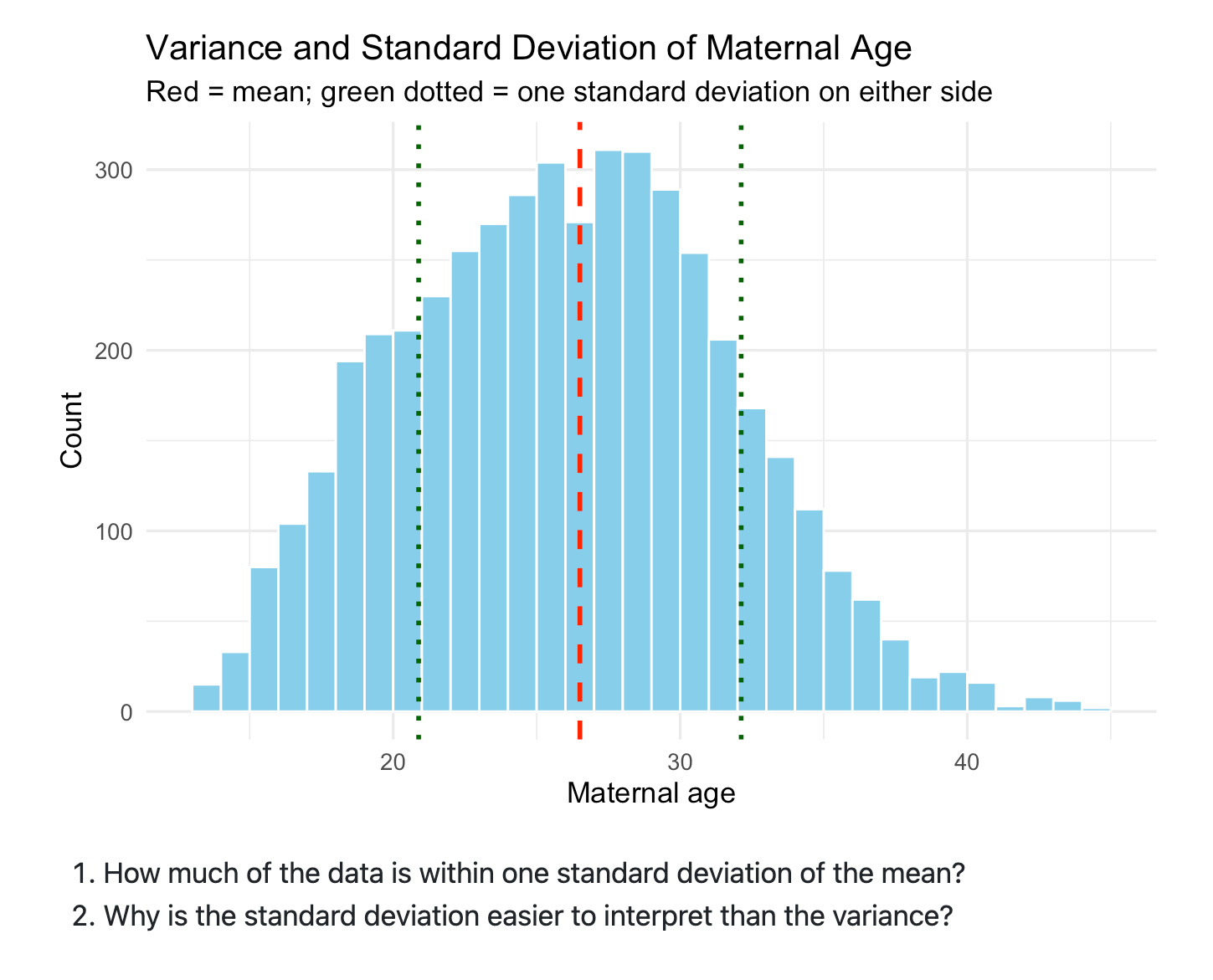
And that is once more how I’m going to introduce confidence intervals — I’m going to pin the idea of variance deep inside them, and solely then transfer into sampling. I’m going to be giving them the analytical equation for calculating commonplace errors, after which I’m going to introduce resampling strategies that additionally give a distribution and since they’ve already seen this image, and the usual deviation, I’m hopeful I can get the concept of the usual error in there too.

It’s onerous to know what’s working and what isn’t as a result of a part of the problem of the category is that it’s 200 college students, whereas Imbens, et al. is 40 college students. So my class is 5 instances bigger, however in any other case, it’s an identical distribution of scholars — freshmen and sophomores primarily, with a thinning tail of juniors and seniors, and with no robust background in stats. I believe if I had a pair goes at it, although, I may nail my model of the course as I’d higher perceive learn how to finest use the “educating fellow” system, which I used to be sluggish to know and use successfully. However subsequent semester, I train a sequel to this course, and I’m in all probability going to emphasise all of the quasi-experimental design strategies, not simply RCT and unconfoundedness. Guido wrote me and stated that artificial management was significantly in style with college students; they understood it rather well. And that has all the time been my expertise educating synth. In reality, I used to inform folks that I believed synth was one of the best ways to assist individuals perceive quasi-experimental design.

The opposite factor I’m doing now’s educating covariate stability tables. I make an enormous deal out of two easy concepts:

1. What’s your remedy group? What’s your management group? What comparability are you making?

2. Have you ever checked in case your covariates are balanced at baseline?

Anyway, I used to be actually inspired after I noticed Imbens, et al. did this as a result of I felt prefer it validated my concept that this might be accomplished, and needs to be accomplished, and extra wanted to be accomplished to determine the pedagogy. There was in all probability a time, in spite of everything, when individuals thought you could possibly solely train calculus at a graduate degree. Then some individuals discovered a method to train it on the undergraduate higher ranges. Then some individuals in all probability discovered methods to inch it earlier. After which lastly somebody discovered a method to stick it into excessive colleges.

I’m within the latter camp. I believe you can too do it with potential outcomes. And I believe you may and may train “causal inference rhetoric” that are tables and figures. And in that, tables exhibiting covariate imbalance needs to be taught consistently. Which has meant additionally educating them a easy software for evaluating teams on covariate stability, particularly the standardized distinction in means.

All that’s simply to say I used to be actually thrilled seeing their class, as I suppose there is part of me that is still insecure about my very own imaginative and prescient of issues. But when Guido Imbens is doing an “early” (i.e., freshmen and sophomores) undergraduate course in causal inference, then rattling straight it’s vital and doable and I’m going to maintain making an attempt to do it. And perhaps one in all nowadays I’ll bug Guido about coauthoring a textbook aimed toward highschool college students.

Reminder about Diff-in-Diff workshop

Altering the topic or a second. However I needed to cancel final weekend’s workshop on diff-in-diff due to my dad’s dying and funeral, however we rescheduled it for subsequent weekend (Nov 15-16 and 22-23). You will discover that info right here.

I’ve been speaking to Kyle about this for some time, however I believe perhaps within the new yr I’m going to start out writing chairs instantly and simply say that in the event that they wish to enroll their total PhD scholar class, we’ll work with them on bulk amount reductions. I stay of the opinion that departments needs to be outsourcing that which they don’t have the time to do on their very own. Coase stated you buy stuff available on the market when the transaction prices to do it your self is just too massive, and so given the huge quantity of econometrics that exist, I don’t see the way it’s doable to show all of it within the few years you may have the scholars. So issues like Mixtape Periods are, for my part, actually essential.

However within the meantime, I’m utilizing my substack and LinkedIn primarily to get the phrase out. So if you wish to find out about diff-in-diff, hit me up. Write me at causalinf@mixtape.consulting in case you assume you might be eligible for a reduction. And in case you are a chair, or know a chair, then ship them this substack and say “hey, let’s get these seats for our college students”. We serve on the pleasure of the king, so to talk. Mixtape Periods offers companies that should shut the worldwide hole between the haves and have-nots in relation to causal inference methodologies, in addition to sometimes different stuff like Jeff and Ariel’s current workshop on structural demand estimation, which was in style as all the time.

Boston

I proceed to like Boston. I’m assembly new individuals. I had a stunning dinner Monday night time for my birthday when a buddy received us tickets to a restaurant on the high of a skyscraper in Again bay, the place I stay. I may see your entire metropolis 360 levels. We walked round exterior in our coats and hats, fingers caught in our pockets, as a result of it was chilly, and simply talked. It was beautiful. Listed here are footage of me turning 50 and blowing out candles.

Neal Cassady as Jack Kerouac’s buddy. And he wrote a guide referred to as “The First Third”. Nicely, I turned 50 and I’m calling it the beginning of “The Second Third” as I believe I’m going to stay to be round 150 years previous sadly. I wouldn’t thoughts giving my children, siblings and mother a few of my years however alas there’s no marketplace for years. So as a substitute I’ll in all probability simply stick round kicking round with my dangerous knees and failing eyesight some time. So right here’s to the second third. Let’s see if I can get well from my failures and pivot the slope of the road up, and shift the intercept approach up. Cheers everybody.