Identification in Artificial Management – by scott cunningham

The figuring out assumption in artificial management that was introduced in Abadie, Diamond and Hainmueller (2010) was that of a “issue mannequin”. I don’t know the historical past of the issue fashions, so I received’t even try, however they appear to be this.

the place Y(0) is the untreated potential end result (e.g., earnings with out some intervention), alpha is a continuing, beta is a time-varying macro-level shock that causes the “returns” to X, some unit-specific observable variable (e.g., agency dimension) to alter over time, mu is a few unit-specific unobservable variable (e.g., CEO means) with mu additionally a time-varying macro-level shock that causes their means’s affect on earnings to range, and a few white noise error time period, varepsilon, that on common is zero.

Let me touch upon just a few issues now. First, the artificial management mannequin initially anyway was extra rooted within the “end result mannequin” custom of identification in that ADH stated one thing alongside the traces of that in case you assumed that all the untreated potential outcomes adopted an element mannequin, then they may have a dialog with you in regards to the bias of artificial management. Put apart for now any updates to this, as Imbens and others have examined the efficiency of artificial management beneath different conditions. For now, simply be aware that.

I name it the end result mannequin custom as a result of that’s form of how my mind works to characterize the other ways of approaching identification within the extra up to date causal inference paradigm. The slang that I hear contrasted to it’s considered one of a randomized therapy project, or design-based strategy, the place one doesn’t specify that the untreated potential end result is characterised any a method, however slightly focuses on the way during which items get assigned to therapy or not (i.e., are they randomized). However artificial management matches extra with difference-in-differences in that an express declare is made, or at the least entertained, that the lacking potential end result follows some acknowledged course of which ADH then use to characterize the bias.

I hesitate to say what I say on this submit for threat I’m mistaken, however I simply needed to share how I perceive this with the caveat that I might be mistaken, so purchaser beware, however I suppose what I’m making an attempt to say is that there are characterizations of potential outcomes and there are characterizations of therapy project processes, and that artificial management initially was extra in step with the end result mannequin identification strategy. And so is diff-in-diff.

Design-based approaches to identification

However that’s the place they differ. The diff-in-diff identification assumption — the essential one anyway — doesn’t want randomization. Certain, randomization of the therapy provides you with parallel tendencies. However randomization of the therapy may also offer you equal imply potential outcomes too. Let’s say that the therapy, D, was impartial of Y(0). Then you may write this down:

I used to seek out it onerous to learn this left to proper for some purpose. I’m not precisely positive what would journey me and I nonetheless don’t. I discovered over time that the one factor that has actually helped me make progress in causal inference has been pencil and paper, writing stuff out, making the deductions myself, and simply working by proofs by hand. That’s the solely factor that basically helps me for small issues and for bigger issues, and maybe an econometrician would say “nicely after all”, however I suppose what I’m saying is that even a line like that must be simple, so within the off probability it isn’t simple, let me clarify.

Independence implies that the therapy is assigned to items “for causes” which have completely nothing to do with that one specific variable known as “the untreated potential end result, Y(0)”. As such, the imply of that variable is similar for each teams, therapy and management. The primary is the imply of potential end result for the handled equal to the second which is the imply of the potential end result for the management to the third which is the imply for the complete pattern. Right here, let me present you utilizing python.

import numpy as np
import matplotlib.pyplot as plt

# Set seed for reproducibility
np.random.seed(42)

# Variety of observations
n = 5000

# Therapy project (impartial of y0)
d = np.random.binomial(1, 0.5, dimension=n)

# Funky y0 course of (imply ≈ 15, sd ≈ 1)
y0 = (
    15
    + np.random.regular(0, 0.8, dimension=n)
    + 0.3 * np.sin(np.random.uniform(0, 2 * np.pi, dimension=n))
)

# Compute means
mean_y0_treated = y0[d == 1].imply()
mean_y0_control = y0[d == 0].imply()
mean_y0_overall = y0.imply()

# Plot
labels = [”E[y0 | d=1]”, “E[y0 | d=0]”, “E[y0]”]
values = [mean_y0_treated, mean_y0_control, mean_y0_overall]

plt.determine()
plt.bar(labels, values)
plt.axhline(mean_y0_overall, linestyle=”--”)
plt.ylabel(”Imply of y0”)
plt.title(”y0 is impartial of therapy”)
plt.present()

See how the means don’t range? That the imply within the therapy group and the imply within the management group are the identical because the imply in the entire pattern? That’s the pattern analog to the inhabitants illustration of Y(0) _||_ D.

The benefit of the design strategy to causal inference is that these deductions are allowed — even when considered one of them doesn’t exist. Are you able to see which of those will be calculated and which of those can’t be calculated? The center one — E[y0|d=0] — is just as soon as we use the switching equation E[y|d=0], the place the switching equation is:

And that’s why you may calculate the center one. You may calculate the center one as a result of for the management group, y(0)=y. So it’s within the information correct, and due to this fact in case you ever want it, you bought it. However the first amount — E[y(0)|d=1] — doesn’t exist as a result of when a unit is handled, we solely observe y(1) by the switching equation. Which suggests we kill off y(0) and thus it doesn’t exist within the information and can by no means exist. It’s misplaced to the ether. It’s a ghost gone to stay with its ancestors in that place the place potential outcomes go after they die earlier than having an opportunity to stay a life.

However right here’s the magic. If the therapy is impartial of y(0), then despite the fact that E[y(0)|d=1] is gone eternally, you continue to have it. You’ve gotten it as a result of it’s equal to E[y(0)|d=0], so anytime alongside this lengthy and windy street you occur to want E[y(0)|d=1], you might have it. It’s simply your useful E[y(0)|d=0]. Because the wizard of Oz tells Dorothy — you have been all the time residence.

Synth Identification Below Random Task and a Issue Mannequin

So then what’s going on with the ADH issue mannequin within artificial management is not historically an announcement in regards to the therapy project. I imply, it’s and it isn’t. If the therapy is actually random, then the anticipated issue fashions could be the identical. If the therapy is random, then in expectation on the inhabitants degree not solely would the y(0) be the identical for therapy and management teams, however so would the underlying construction on the right-hand facet. I made one other python script with random therapy project so you may see it, and I “jiggled” the traces in order that they’d be separated barely aside on the graph. After which I ran a Monte Carlo simulation the place I repeated the producing of the information by the issue mannequin processes 1,000 occasions, plotted the imply line, and plotted the usual deviation multiplied by 1.96 so you might see the 95% confidence intervals too. I additionally made it in order that the y(0) is killed off post-treatment for the therapy group however not the management group. Notice, I solely jiggled it so that you’d see it on the identical graph, however in actuality in expectation the inhabitants could be the identical on common.

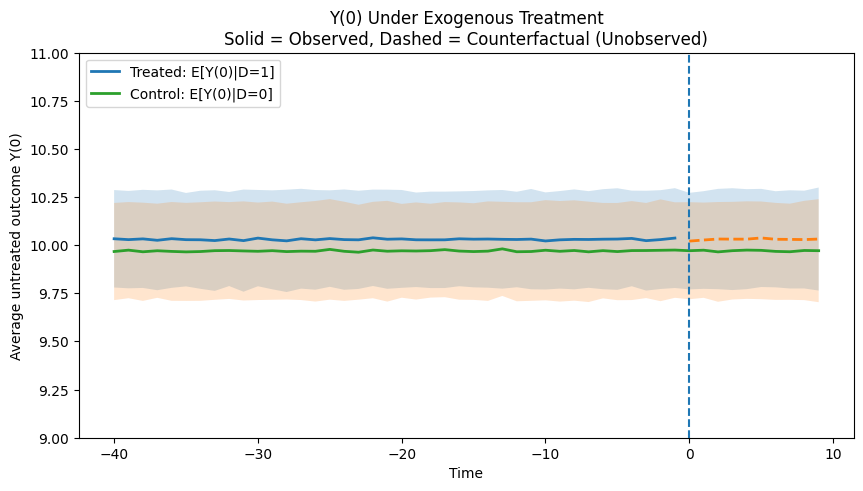
With the code in python once more right here:

import numpy as np
import matplotlib.pyplot as plt

np.random.seed(123)

# Parameters
n_units = 500
T_pre = 40
T_post = 10
T = T_pre + T_post
years = np.arange(-T_pre, T_post)
n_mc = 1000

alpha = 10
sigma_eps = 2

treated_paths = np.zeros((n_mc, T))
control_paths = np.zeros((n_mc, T))

for m in vary(n_mc):
    X = np.random.regular(0, 1, n_units)
    mu = np.random.regular(0, 1, n_units)
    D = np.random.binomial(1, 0.5, n_units)

    beta_t = 0.2 + 0.005 * years
    omega_t = 0.4 + 0.02 * np.cos(years / 6)

    Y0 = np.zeros((n_units, T))
    for t in vary(T):
        eps = np.random.regular(0, sigma_eps, n_units)
        Y0[:, t] = alpha + beta_t[t] * X + omega_t[t] * mu + eps

    Y0_obs = Y0.copy()
    post_idx = years >= 0
    Y0_obs[D == 1, :][:, post_idx] = np.nan

    treated_paths[m, :] = np.nanmean(Y0_obs[D == 1], axis=0)
    control_paths[m, :] = Y0_obs[D == 0].imply(axis=0)

treated_mean = np.nanmean(treated_paths, axis=0)
control_mean = control_paths.imply(axis=0)

treated_sd = np.nanstd(treated_paths, axis=0)
control_sd = control_paths.std(axis=0)

# small visible offset
treated_mean = treated_mean + 0.03
control_mean = control_mean - 0.03

plt.determine(figsize=(10, 5))

# Pre-treatment stable, post-treatment dashed for handled Y(0)
pre = years < 0
submit = years >= 0

plt.plot(years[pre], treated_mean[pre], label=”Handled: E[Y(0)|D=1]”, linewidth=2)
plt.plot(years[post], treated_mean[post], linestyle=”--”, linewidth=2)

plt.plot(years, control_mean, label=”Management: E[Y(0)|D=0]”, linewidth=2)

plt.fill_between(
    years,
    treated_mean - 1.96 * treated_sd,
    treated_mean + 1.96 * treated_sd,
    alpha=0.2,
)

plt.fill_between(
    years,
    control_mean - 1.96 * control_sd,
    control_mean + 1.96 * control_sd,
    alpha=0.2,
)

plt.axvline(0, linestyle=”--”)
plt.ylim(9, 11)
plt.xlabel(”Time”)
plt.ylabel(”Common untreated end result Y(0)”)
plt.title(
    “Y(0) Below Exogenous TreatmentnSolid = Noticed, Dashed = Counterfactual (Unobserved)”
)
plt.legend()
plt.present()

Skiping over how artificial management does its calculations, be aware that what it turns into is that this:

the place the primary time period is the y(0) for the one handled unit, and the second is the artificial management the place the weights are on the management group, w_j. Below randomization, these two portions are the identical. But when they’re the identical, then it implies that the RHS would even be the identical:

And so just a few issues occur. First, the fixed, alpha, is deleted. Second, the observables are comparable on common in order that first time period will get deleted no matter beta, and on all the way down to the precise. And on this case, you might use any set of weights as a result of the typical of any weighted group can be on common equal to that of the handled unit’s personal time path pre-treatment. At the very least within the frequentist sense the place the items are random attracts from some tremendous inhabitants.

However right here’s the factor. Below random project, we don’t want to care in regards to the issue mannequin itself. We don’t even have to make the idea that it did observe that course of. And we don’t want artificial management as a result of beneath randomized therapy project, we simply all the time can deduce that the

Synth Identification Below Non-Randomized Therapy Task

In order that’s type of the design strategy to identification. The whole lot robotically cancels out beneath no matter central restrict theorem we invoke. However what if don’t have random project? Properly, if we don’t have random project, then we can not simply assume that the means are impartial of therapy project. Which suggests then that these weights really will matter an excellent deal. First, let me write down the issue mannequin once more:

And now let me write down the bias of the artificial management (once more, skipping the place it got here from) because the distinction between the handled unit (unit 1) and the weighted common of the J management group items:

And once I write that down noting the left hand then the precise hand facet additionally will get differenced and it’s right here:

Properly, artificial management is all about “matching nicely”, and right here think about it was estimated by matching on the observable X. You’ll usually use lagged outcomes for that, however for now simply be basic about it and simply be aware that we’ve got some course of the place X causes Y(0). So then let’s assume you probably did “match nicely” on the observable. That might then imply this:

This causes the primary time period, which be aware is a residual of kinds, to be roughly zero:

And I deleted it as a result of we will really verify that. However then that leaves us with two extra phrases, neither of which we will verify, as mu shouldn’t be observable (recall it’s the CEO’s unobserved means) and varepsilon are these random shocks. And that’s roughly the bias. The bias of artificial management of ADH is the matching bias related to mu and differential however what they name “transitory shocks” such that there’s additionally a residual hole there. And that’s mainly the bias roughly.

Principally, ADH explicitly say that in case you might match each noticed covariates, X, and the unobserved issue “loadings” that are these time-varying processes on it, beta, you’d be unbiased so lengthy the time-varying loadings in your unobserved mu additionally matched, in addition to the residuals on these transitory shocks.

Properly that is the place you begin to notice what synth is doing and the way it isn’t so simple as the plug-and-play you get from independence. You may’t assume these are the identical in any weighted common within the course of. The weights, slightly, matter, nevertheless it’s not simply that. It should be the case that management group items exist within the information that observe the identical course of and which when weighted are in reality comparable. Synth “finds” them observationally by matching on X, ideally the lagged Y outcomes although since the most effective predictor of future Y(0) is most definitely the previous, even when that Y(0) is killed off.

However again to my level. Since mu isn’t noticed, that is the place the ADH argument is available in: an extended pre-period + good pre-fit of outcomes makes it onerous to get that match except mu can also be roughly matched—in any other case you’d be counting on varepsilon “simply so” to compensate (overfitting). That is the place you’ll typically hear a phrase when individuals talk about artificial management — are you matching on the “construction” (that means the loadings and the unobserved heterogeneity, mu) or are you “matching on noise”?

In a short-panel, you’d solely be protected if the transitory shocks are roughly approaching zero, which isn’t knowable, as long as there did exist “good matches” within the information (i.e., for which Xs are matched nicely). However you may’t be certain and that’s why, within the Journal of Financial Literature primer on synth by Abadie (2021), the sensible “bias management” dialogue is framed across the “scale of the transitory shocks” and the size of the pre-period (often stated with notation T_0).

And that is it. That’s the identification. It’s the issue mannequin driving it.

Conclusion

So, how does this evaluate with diff-in-diff? Properly, apparently, they’re totally different and comparable with respect to their figuring out assumptions to a level. Technically, parallel tendencies doesn’t “want” the lengthy pre-treatment. Diff-in-diff makes use of the pre-treatment coefficients within the 2xT occasion research to argue that parallel tendencies within the post-treatment is an affordable perception to carry, however you may establish the ATT with a diff-in-diff with a easy 2×2 (i.e., just one pre-treatment interval). It’s possible you’ll not discover it convincing with out seeing the occasion examine, however that’s not identification. That’s falsification.

So then, does artificial management “want” the lengthy pre-treatment? Properly, form of. I imply, you might use artificial management with a one interval. You’d remedy that constrained distance minimization operate, get your non-negative weights, after which run them ahead to get dynamic estimated therapy results. So in that sense, no you don’t “want” the lengthy collection.

My studying is totally different. My studying is that it’s comparable in that I feel beneath the issue mannequin, we will acquire extra confidence that we’ve got a weighted common with those self same two residual phrases (on the heterogeneity and on the transitory shocks). So in a way, I feel it’s most likely bought the same operate because the 2xT occasion examine, although I’m positive others could disagree, and albeit I feel I modified my opinion on this in the middle of this substack and after I take my bathe, I could change again, however my level is that you just’re assuming an element mannequin of Y(0), you’re hoping and praying that a few items at the least within the donor pool are comparable sufficient on that underlying construction that artificial management can discover them with that distance minimization method, and also you’re extra probably to try this with the lengthy than the quick pre-treatment time collection resulting from that idiosyncratic error in there that can also be contributing to the bias.

Alberto Abadie, Basque, and Historical past of Thought Fast Detour

Anyway, that’s my understanding of identification with the artificial management mannequin. All errors are my very own. Thanks once more to my favourite econometrician, Alberto Abadie, for his contributions to causal inference going all the best way again to being Josh Angrist’s scholar at MIT — considered one of his first, a classmate in Josh’s second cohort with such luminaries as Sue Dynarski, Jonah Gelbach, Marianne Bitler, and Esther Duflo. I feel there’s a sixth, and I appear to keep in mind that Jeff Kling possibly was Josh’s first scholar (a singleton) who graduated earlier than that second cohort, however I’m drawing a clean on that individual’s identify. It’s buried in my notes someplace.

However anyway, my level is, Alberto got here out swinging, making authentic contributions to just about no matter he touched whether or not it was instrumental variables (that’s the place we get kappa weights which turned out to be influential within the decide designs due to the flexibility to get complier traits, which you’ll now an increasing number of seen executed, most likely partly because of Peter Hull (one other considered one of my favourite econometricians, and likewise a Josh scholar) pushing for it, and selling that earlier Abadie work. Then Alberto goes on a tear working with Guido Imbens on matching associated matters. Just about instantly, Alberto goes to Basque Nation on the invitation of Javier Gardeazabal to do a workshop the place the 2 of them talked about doing a venture collectively in regards to the impact of the ETA terrorist group on combination revenue. And that’s the place Alberto cooked up artificial management, and in a podcast once I requested him about it, like why did he give you it, the very first thing he instructed me was as a result of he beloved his residence within the Basque Nation. A remark I nonetheless take into consideration to today — what a pleasant thought that love led to one of the vital essential improvements in causal inference of the final 25 years.

Basque Nation — that romantic, lovely area in Northern Spain. An autonomous area I’ve now visited two summers in a row. I went as much as a vendor close to the seaside as soon as and after they requested me why I had come to go to lovely San Sebastián (as if somebody wants a purpose to go to San Sebastián), I instructed them this was the place my favourite econometrician was from. After which jokingly I instructed them “and this was the place artificial management was born”. Since I don’t converse Spanish, however slightly I converse the thick dialect of deep Mississippi, I’m positive that made as a lot sense to them as the rest I stated.

Anyway, I wakened this morning wanting to put in writing all this down. My semester is winding down. It’s been the toughest semester of my whole life. There’s in reality no artificial management I might create for it if I drew from each different earlier semester in my very own 25 years of educating. I imply, I might do it. You may all the time get a weighted common of management group items that reduce a long way operate that minimizes the squared sum of matching discrepancies. I simply could be I the outlier and means, means off the convex hull. However that’s for one more substack for one more day, possibly one other yr, an outdated man.

Comfortable holidays. And bear in mind, don’t overlook to place Sufjan Stevens Christmas album on this yr, at the least as soon as. I really self medicate my stress ranges listening to it, having moved away from hip hop and various music, as Cosmos stated I wanted to do extra grounding workout routines and actually really useful it to me.