

New to Stata 14 is a set of instructions to suit merchandise response principle (IRT) fashions. IRT fashions are used to research the connection between the latent trait of curiosity and the gadgets meant to measure the trait. Stata’s irt instructions present quick access to a number of the generally used IRT fashions for binary and polytomous responses, and irtgraph instructions can be utilized to plot merchandise attribute features and data features.
To be taught extra about Stata’s IRT options, I refer you to the [IRT] guide; right here I wish to transcend the guide and present you a few examples of what you are able to do with a little bit little bit of Stata code.
Instance 1
To get began, I wish to present you ways easy IRT evaluation is in Stata.
Once I use the 9 binary gadgets q1–q9, all I must sort to suit a 1PL mannequin is
irt 1pl q*
Equivalently, I can use a touch notation or explicitly spell out the variable names:
irt 1pl q1-q9
irt 1pl q1 q2 q3 this autumn q5 q6 q7 q8 q9
I can even use parenthetical notation:
irt (1pl q1-q9)
Parenthetical notation shouldn’t be very helpful for a easy IRT mannequin, however is useful if you wish to match a single IRT mannequin to combos of binary, ordinal, and nominal gadgets:
irt (1pl q1-q5) (1pl q6-q9) (pcm x1-x10) ...
IRT graphs are equally easy to create in Stata; for instance, to plot merchandise attribute curves (ICCs) for all of the gadgets in a mannequin, I sort
irtgraph icc
Sure, that’s it!
Instance 2
Generally, I wish to match the identical IRT mannequin on two completely different teams and see how the estimated parameters differ between the teams. The train could be a part of investigating differential merchandise functioning (DIF) or parameter invariance.
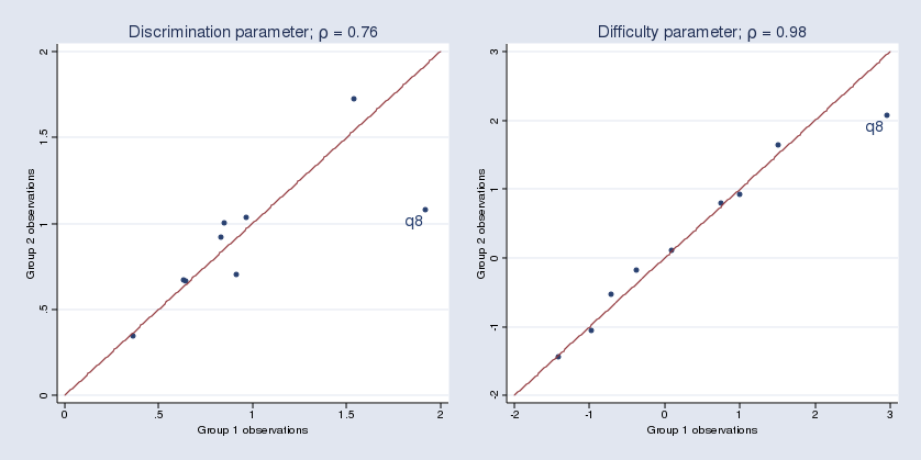
I cut up the info into two teams, match two separate 2PL fashions, and create two scatterplots to see how shut the parameter estimates for discrimination and issue are for the 2 teams. For simplicity, my group variable is 1 for odd-numbered observations and 0 for even-numbered observations.
We see that the estimated parameters for merchandise q8 seem to vary between the 2 teams.
Right here is the code used on this instance.
webuse masc1, clear

gen odd = mod(_n,2)

irt 2pl q* if odd
mat b_odd = e(b)'

irt 2pl q* if !odd
mat b_even = e(b)'

svmat double b_odd, names(group1)
svmat double b_even, names(group2)
substitute group11 = . in 19
substitute group21 = . in 19

gen lab1 = ""
substitute lab1 = "q8" in 15

gen lab2 = ""
substitute lab2 = "q8" in 16

corr group11 group21 if mod(_n,2)
native c1 : show %4.2f `r(rho)'

twoway (scatter group11 group21, mlabel(lab1) mlabsize(giant) mlabpos(7)) ///
        (operate x, vary(0 2)) if mod(_n,2), ///
        identify(discr,substitute) title("Discrimination parameter; {&rho} = `c1'") ///
        xtitle("Group 1 observations") ytitle("Group 2 observations") ///
        legend(off)

corr group11 group21 if !mod(_n,2)
native c2 : show %4.2f `r(rho)'

twoway (scatter group11 group21, mlabel(lab2) mlabsize(giant) mlabpos(7)) ///
        (operate x, vary(-2 3)) if !mod(_n,2), ///
        identify(diff,substitute) title("Problem parameter; {&rho} = `c2'") ///
        xtitle("Group 1 observations") ytitle("Group 2 observations") ///
        legend(off)

graph mix discr diff, xsize(8)
Instance 3
Persevering with with the instance above, I wish to present you use a likelihood-ratio take a look at to check for merchandise parameter variations between teams.
Utilizing merchandise q8 for instance, I wish to match one mannequin that constrains merchandise q8 parameters to be the identical between the 2 teams and match one other mannequin that enables these parameters to range.
The primary mannequin is simple. I can match a 2PL mannequin for your entire dataset, which implicitly constrains the parameters to be equal for each teams. I retailer the estimates beneath the identify equal.
. webuse masc1, clear
(Knowledge from De Boeck & Wilson (2004))

. generate odd = mod(_n,2)
. quietly irt 2pl q*
. estimates retailer equal
To estimate the second mannequin, I would like the next:
. irt (2pl q1-q7 q9) (2pl q8 if odd) (2pl q8 if !odd)
Sadly, that is unlawful syntax. I can, nevertheless, cut up the merchandise into two new variables the place every variable is restricted to the required subsample:
. generate q8_1 = q8 if odd
(400 lacking values generated)

. generate q8_2 = q8 if !odd
(400 lacking values generated)
I estimate the second IRT mannequin, this time with gadgets q8_1 and q8_2 going down of the unique q8:
. quietly irt 2pl q1-q7 q8_1 q8_2 q9
. estat report q8_1 q8_2

Two-parameter logistic mannequin                    Variety of obs     =        800
Log chance = -4116.2064
------------------------------------------------------------------------------
             |      Coef.   Std. Err.      z    P>|z|     [95% Conf. Interval]
-------------+----------------------------------------------------------------
q8_1         |
     Discrim |   1.095867   .2647727     4.14   0.000     .5769218    1.614812
        Diff |  -1.886126   .3491548    -5.40   0.000    -2.570457   -1.201795
-------------+----------------------------------------------------------------
q8_2         |
     Discrim |    1.93005   .4731355     4.08   0.000     1.002721    2.857378
        Diff |  -1.544908   .2011934    -7.68   0.000     -1.93924   -1.150577
------------------------------------------------------------------------------
Now, I can carry out the likelihood-ratio take a look at:
. lrtest equal ., drive

Chance-ratio take a look at                                 LR chi2(2)  =      4.53
(Assumption: equal nested in .)                       Prob > chi2 =    0.1040
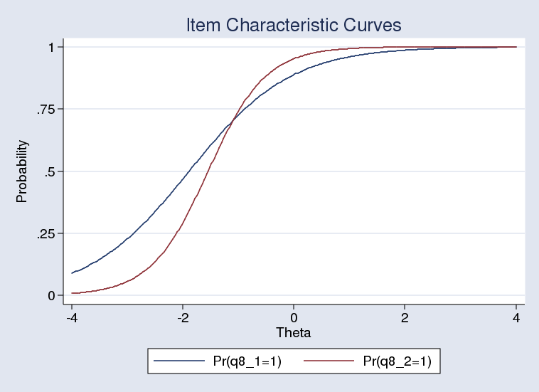
The take a look at suggests the primary mannequin is preferable regardless that the 2 ICCs clearly differ:
. irtgraph icc q8_1 q8_2, ylabel(0(.25)1)
Abstract
IRT fashions are used to research the connection between the latent trait of curiosity and the gadgets meant to measure the trait. Stata’s irt instructions present quick access to a number of the generally used IRT fashions, and irtgraph instructions implement probably the most generally used IRT plots. With just some further steps, you possibly can simply create personalized graphs, resembling those demonstrated above, which incorporate info from separate IRT fashions.