Finite Combination Mannequin primarily based on Dirichlet Distribution

This weblog put up is the second a part of an article collection on Dirichlet Course of combination fashions. Within the earlier article we had an overview of a number of Cluster Evaluation methods and we mentioned a number of the issues/limitations that rise by utilizing them. Furthermore we briefly introduced the Dirichlet Course of Combination Fashions, we talked about why they’re helpful and we introduced a few of their functions.

Replace: The Datumbox Machine Studying Framework is now open-source and free to obtain. Try the bundle com.datumbox.framework.machinelearning.clustering to see the implementation of Dirichlet Course of Combination Fashions in Java.

The Dirichlet Course of Combination Fashions is usually a bit exhausting to swallow in the beginning primarily as a result of they’re infinite combination fashions with many alternative representations. Happily a great way to method the topic is by ranging from the Finite Combination Fashions with Dirichlet Distribution after which shifting to the infinite ones.

Consequently on this article I’ll briefly current some essential distributions that we’ll want, we are going to use them to assemble the Dirichlet Prior with Multinomial Chance mannequin after which we are going to transfer to the Finite Combination Mannequin primarily based on the Dirichlet Distribution.

1. Beta Distribution

The Beta distribution is a household of steady distributions which is outlined within the interval of [0,1]. It’s parameterized by two optimistic parameters a and b and its type closely relies upon upon the number of these two parameters.

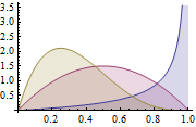
Determine 1: Beta Distribution for various a, b parameters

The Beta distribution is often used to mannequin a distribution over possibilities and has the next likelihood density:

Equation 1: Beta PDF

The place Γ(x) is the gamma operate and a, b the parameters of the distribution. Beta is often used as a distribution of likelihood values and offers us the chance that the modelled likelihood equals to a selected worth P = p0. By its definition Beta distribution is ready to mannequin the likelihood of binary outcomes which take values true or false. The parameters a and b might be thought of because the pseudocounts of success and failure respectively. Thus the Beta Distribution fashions the likelihood of success given a successes and b failures.

2. Dirichlet Distribution

The Dirichlet Distribution is the generalisation of Beta Distribution for a number of outcomes (or in different phrases it’s used for occasions with a number of outcomes). It’s parameterized with okay parameters a_i which should be optimistic. Dirichlet Distribution equals to the Beta Distribution when the variety of variables okay = 2.

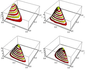
Determine 2: Dirichlet Distribution for numerous a_i parameters

The Dirichlet distribution is often used to mannequin a distribution over possibilities and has the next likelihood density:

Equation 2: Dirichlet PDF

The place Γ(x) is the gamma operate, the p_i take values in [0,1] and Σp_i=1. The Dirichlet distribution fashions the joint distribution of p_i and offers the chance of P₁=p₁,P₂=p₂,….,P_k-1=p_k-1 with P_okay=1 – ΣP_i. As within the case of Beta, the a_i parameters might be thought of as pseudocounts of the appearances of every i occasion. The Dirichlet distribution is used to mannequin the likelihood of okay rival occasions occurring and is commonly denoted as Dirichlet(a).

3. Dirichlet Prior with Multinomial Chance

As talked about earlier the Dirichlet distribution might be seen as a distribution over likelihood distributions. In circumstances the place we wish to mannequin the likelihood of okay occasions occurring, a Bayesian method could be to make use of Multinomial Chance and Dirichlet Priors .

Under we are able to see the graphical mannequin of such a mannequin.

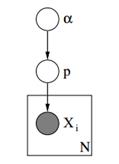
Determine 3: Graphical Mannequin of Dirichlet Priors with Multinomial Chance

Within the above graphical mannequin, α is a okay dimensional vector with the hyperparameters of Dirichlet priors, p is a okay dimensional vector with the likelihood values and x_i is a scalar worth from 1 to okay which tells us which occasion has occurred. Lastly we should always be aware that the P follows the Dirichlet distribution parameterized with vector α and thus P ~ Dirichlet(α), whereas the x_i variables observe the Discrete distribution (Multinomial) parameterized with the p vector of possibilities. Related hierarchical fashions can be utilized in doc classification to characterize the distributions of key phrase frequencies for in numerous subjects.

4. Finite Combination Mannequin with Dirichlet Distribution

Through the use of Dirichlet Distribution we are able to assemble a Finite Combination Mannequin which can be utilized to carry out clustering. Let’s assume that we have now the next mannequin:

Equation 3: Finite Combination Mannequin with Dirichlet Distribution

The above mannequin assumes the next: We have now a dataset X with n observations and we wish to carry out cluster evaluation on it. The okay is a continuing finite quantity which reveals the variety of clusters/parts that we’ll use. The c_i variables retailer the cluster task of remark X_i, they take values from 1 to okay and observe the Discrete Distribution with parameter p that are the combination possibilities of the parts. The F is the generative distribution of our X and it’s parameterized with a parameter which is dependent upon the cluster task of every remark. In whole we have now okay distinctive parameters equal to the variety of our clusters. The variable shops the parameters that parameterize the generative F Distribution and we assume that it follows a base G₀ distribution. The p variable shops the combination percentages for each one of many okay clusters and follows the Dirichlet with parameters α/okay. Lastly the α is a okay dimensional vector with the hyperparameters (pseudocounts) of Dirichlet distribution [2].

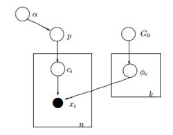
Determine 4: Graphical Mannequin of Finite Combination Mannequin with Dirichlet Distribution

A less complicated and fewer mathematical solution to clarify the mannequin is the next. We assume that our information might be grouped in okay clusters. Every cluster has its personal parameters and people parameters are used to generate our information. The parameters are assumed to observe some distribution G₀. Every remark is represented with a vector x_i and a c_i worth which signifies the cluster to which it belongs. Consequently the c_i might be seen as a variable which follows the Discrete Distribution with a parameter p which is nothing however the combination possibilities, i.e. the likelihood of the prevalence of every cluster. Provided that we deal with our downside in a Bayesian approach, we don’t deal with the parameter p as a continuing unknown vector. As a substitute we assume that the P follows Dirichlet which is parameterized by hyperparameters α/okay.

5. Working with infinite okay clusters

The earlier combination mannequin permits us to carry out unsupervised studying, follows a Bayesian method and might be prolonged to have a hierarchical construction. Nonetheless it’s a finite mannequin as a result of it makes use of a continuing predefined okay variety of clusters. Consequently it requires us to outline the variety of parts earlier than performing Cluster Evaluation and as we mentioned earlier in most functions that is unknown and may’t be simply estimated.

One solution to resolve that is to think about that okay has a really giant worth which tends to infinity. In different phrases we are able to think about the restrict of this mannequin when okay tends to infinity. If so, then we are able to see that regardless of that the variety of clusters okay is infinite, the precise variety of clusters which might be lively (those which have no less than one remark), can’t be bigger than n (which is the entire variety of the observations in our dataset). In truth as we are going to see later, the variety of lively clusters might be considerably lower than n and they are going to be proportional to .

After all taking the restrict of okay to infinity is non-trivial. A number of questions rise akin to whether or not it’s potential to take such a restrict, how would this mannequin appear like and how can we assemble and use such a mannequin.

Within the subsequent article we are going to deal with precisely these questions: we are going to outline the Dirichlet Course of, we are going to current the assorted representations of DP and eventually we are going to deal with the Chinese language Restaurant Course of which is an intuitive and environment friendly solution to assemble a Dirichlet Course of.

I hope you discovered this put up helpful. Should you did please take a second to share the article on Fb and Twitter. 🙂